Changhyoni_developer

### 2021.12.18

• NumPy의 배열 연산은 벡터화(vectorized) 연산을 사용
• 일반적으로 NumPy의 범용 함수(universal functions)를 통해 구현
• 배열 요소에 대한 반복적인 계산을 효율적으로 수행

브로드캐스팅(Broadcasting)

#In[]
import numpy as np

a1 = np.array([1,2,3])
print(a1)
print(a1 + 5)

#Out[]
[1 2 3]

[6 7 8]

#In[]
a2 = np.arange(1,10).reshape(3,3)
print(a2)
print(a1 + a2)

#Out[]
[[1 2 3]
 [4 5 6]
 [7 8 9]]
 
[[ 2  4  6]
 [ 5  7  9]
 [ 8 10 12]]

#In[]
b2 = np.array([1,2,3]).reshape(3,1)
print(b2)
print(a1 + b2)

#Out[]
[[1]
 [2]
 [3]]
 
[[2 3 4]
 [3 4 5]
 [4 5 6]]

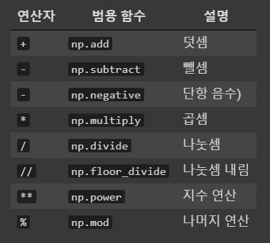
산술 연산(Arithmetic Operators)

#In[]
a1 = np.arange(1,10)
print(a1)
print(a1 + 1)
print(np.add(a1, 10))

#Out[]
[1 2 3 4 5 6 7 8 9]
[ 2  3  4  5  6  7  8  9 10]
[11 12 13 14 15 16 17 18 19]

#In[]
print(a1 - 2)
print(np.subtract(a1, 10))

#Out[]
[-1  0  1  2  3  4  5  6  7]
[-9 -8 -7 -6 -5 -4 -3 -2 -1]

#In[]
print(-a1)
print(np.negative(a1))

#Out[]
[-1 -2 -3 -4 -5 -6 -7 -8 -9]
[-1 -2 -3 -4 -5 -6 -7 -8 -9]

#In[]
print(a1 * 2)
print(np.multiply(a1, 2))

#Out[]
[ 2  4  6  8 10 12 14 16 18]
[ 2  4  6  8 10 12 14 16 18]

#In[]
print(a1 / 2)
print(np.divide(a1, 2))

#Out[]
[0.5 1.  1.5 2.  2.5 3.  3.5 4.  4.5]
[0.5 1.  1.5 2.  2.5 3.  3.5 4.  4.5]

#In[]
print(a1 // 2)
print(np.floor_divide(a1,2))

#Out[]
[0 1 1 2 2 3 3 4 4]
[0 1 1 2 2 3 3 4 4]

#In[]
print(a1 ** 2)
print(np.power(a1, 2))

#Out[]
[ 1  4  9 16 25 36 49 64 81]
[ 1  4  9 16 25 36 49 64 81]

#In[]
print(a1 % 2)
print(np.mod(a1,2))

#Out[]
[1 0 1 0 1 0 1 0 1]
[1 0 1 0 1 0 1 0 1]

# 배열간의 연산도 가능하다
#In[]
a1 = np.arange(1, 10)
print(a1)

b1 =  np.random.randint(1, 10, size=9)
print(b1)

print(a1 + b1)
print(a1 - b1)
print(a1 * b1)
print(a1 / b1)
print(a1 // b1)
print(a1 ** b1)
print(a1 % b1)

#Out[]
[1 2 3 4 5 6 7 8 9]
[7 8 8 6 6 5 1 7 1]
[ 8 10 11 10 11 11  8 15 10]
[-6 -6 -5 -2 -1  1  6  1  8]
[ 7 16 24 24 30 30  7 56  9]
[0.14285714 0.25       0.375      0.66666667 0.83333333 1.2
 7.         1.14285714 9.        ]
[0 0 0 0 0 1 7 1 9]
[      1     256    6561    4096   15625    7776       7 2097152       9]
[1 2 3 4 5 1 0 1 0]

# 2차원에서도 가능!!
#In[]
a2 = np.arange(1,10).reshape(3,3)
print(a2)

b2 = np.random.randint(1, 10, size=(3,3))
print(b2)

print(a2 + b2)
print(a2 - b2)

#Out[]
[[1 2 3]
 [4 5 6]
 [7 8 9]]
 
[[4 6 3]
 [4 7 3]
 [4 4 8]]
 
[[ 5  8  6]
 [ 8 12  9]
 [11 12 17]]
 
[[-3 -4  0]
 [ 0 -2  3]
 [ 3  4  1]]

  절대값 함수(Absolute Function)

• absolute(), abs(): 내장된 절대값 함수

#In[]
a1 = np.random.randint(-10, 10, size=5)
print(a1)
print(np.absolute(a1))
print(np.abs(a1))

#Out[]
[-10   5   2  -9   2]
[10  5  2  9  2]
[10  5  2  9  2]

 제곱/제곱근 함수

• square, sqrt: 제곱, 제곱근 함수

#In[]
print(a1)
print(np.square(a1))
print((np.sqrt(np.abs(a1))))

#Out[]
[-10   5   2  -9   2]
[100  25   4  81   4]
[3.16227766 2.23606798 1.41421356 3.         1.41421356]

지수와 로그 함수 (Exponential and Log Function)

#In[]
a1 = np.random.randint(1, 10, size=5)
print(a1)
print(np.exp(a1))
print(np.exp2(a1))
print(np.power(a1,2))

#Out[]
[1 6 2 1 9]
[2.71828183e+00 4.03428793e+02 7.38905610e+00 2.71828183e+00
 8.10308393e+03]
[  2.  64.   4.   2. 512.]
[ 1 36  4  1 81]

#In[]
print(a1)
print(np.log(a1))
print(np.log2(a1))
print(np.log10(a1))

#Out[]
[1 6 2 1 9]
[0.         1.79175947 0.69314718 0.         2.19722458]
[0.        2.5849625 1.        0.        3.169925 ]
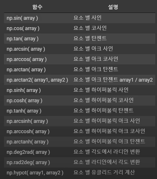
[0.         0.77815125 0.30103    0.         0.95424251]

삼각 함수(Trigonometrical Function)

#In[]
t = np.linspace(0, np.pi, 3)

print(t)
print(np.sin(t))
print(np.cos(t))
print(np.tan(t))

#Out[]
[0.         1.57079633 3.14159265]
[0.0000000e+00 1.0000000e+00 1.2246468e-16]
[ 1.000000e+00  6.123234e-17 -1.000000e+00]
[ 0.00000000e+00  1.63312394e+16 -1.22464680e-16]

#In[]
x = [-1, 0, 1]
print(x)
print(np.arcsin(x))
print(np.arccos(x))
print(np.arctan(x))

#Out[]
[-1, 0, 1]
[-1.57079633  0.          1.57079633]
[3.14159265 1.57079633 0.        ]
[-0.78539816  0.          0.78539816]

집계 함수(Aggregate Functions)

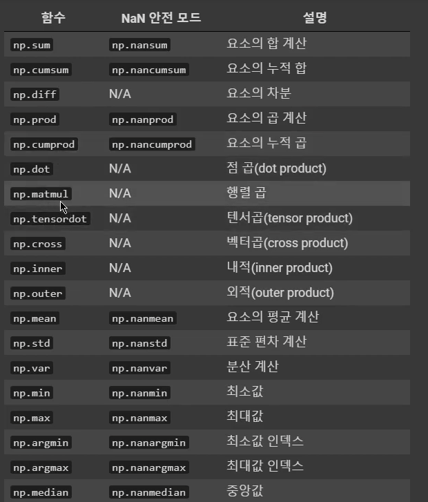
sum(): 합 계산

#In[]
a2 = np.random.randint(1, 10, size=(3,3))
print(a2)
print(a2.sum(), np.sum(a2))
print(a2.sum(axis=0), np.sum(a2, axis=0))
print(a2.sum(axis=1), np.sum(a2, axis=1))

#Out[]
[[2 2 7]
 [4 5 6]
 [2 7 4]]
39 39
[ 8 14 17] [ 8 14 17]
[11 15 13] [11 15 13]

cumsum(): 누적합 계산

#In[]
print(a2)
print(np.cumsum(a2))
print(np.cumsum(a2, axis=0))
print(np.cumsum(a2, axis=1))

#Out[]
[[2 2 7]
 [4 5 6]
 [2 7 4]]
 
[ 2  4 11 15 20 26 28 35 39]

[[ 2  2  7]
 [ 6  7 13]
 [ 8 14 17]]
 
[[ 2  4 11]
 [ 4  9 15]
 [ 2  9 13]]

diff(): 차분 계산

#In[]
print(a2)
print(np.diff(a2))
print(np.diff(a2, axis=0))
print(np.diff(a2, axis=1))

#Out[]
[[2 2 7]
 [4 5 6]
 [2 7 4]]
 
[[ 0  5]
 [ 1  1]
 [ 5 -3]]
 
[[ 2  3 -1]
 [-2  2 -2]]
 
[[ 0  5]
 [ 1  1]
 [ 5 -3]]

 prod(): 곱 계산

#In[]
print(a2)
print(np.prod(a2))
print(np.prod(a2, axis=0))
print(np.prod(a2, axis=1))

#Out[]
[[2 2 7]
 [4 5 6]
 [2 7 4]]
 
188160

[ 16  70 168]

[ 28 120  56]

cumprod(): 누적곱 계산

#In[]
print(a2)
print(np.cumprod(a2))
print(np.cumprod(a2, axis=0))
print(np.cumprod(a2, axis=1))

#Out[]
[[2 2 7]
 [4 5 6]
 [2 7 4]]
 
[     2      4     28    112    560   3360   6720  47040 188160]

[[  2   2   7]
 [  8  10  42]
 [ 16  70 168]]
 
[[  2   4  28]
 [  4  20 120]
 [  2  14  56]]

dot()/matmul(): 점곱/행렬곱 계산

#In[]
b2 = np. ones_like(a2)
print(a2)
print(b2)

print(np.dot(a2, b2))
print(np.matmul(a2, b2))

#Out[]
[[2 2 7]
 [4 5 6]
 [2 7 4]]
[[1 1 1]
 [1 1 1]
 [1 1 1]]
 
[[11 11 11]         # 2*1 + 2*1 + 7*1
 [15 15 15]         # 4*1 + 5*1 + 6*1
 [13 13 13]]        # 2*1 + 7*1 + 4*1
 
[[11 11 11]
 [15 15 15]
 [13 13 13]]

tensordot(): 텐서곱 계산

#In[]
print(a2)
print(b2)

print(np.tensordot(a2,b2))
print(np.tensordot(a2,b2, axes=0))
print(np.tensordot(a2,b2, axes=1))

#Out[]
[[2 2 7]
 [4 5 6]
 [2 7 4]]
[[1 1 1]
 [1 1 1]
 [1 1 1]]
 
39             #행렬곱하고 더하기!

[[[[2 2 2]     
   [2 2 2]
   [2 2 2]]

  [[2 2 2]
   [2 2 2]
   [2 2 2]]

  [[7 7 7]
   [7 7 7]
   [7 7 7]]]


 [[[4 4 4]
   [4 4 4]
   [4 4 4]]

  [[5 5 5]
   [5 5 5]
   [5 5 5]]

  [[6 6 6]
   [6 6 6]
   [6 6 6]]]


 [[[2 2 2]
   [2 2 2]
   [2 2 2]]

  [[7 7 7]
   [7 7 7]
   [7 7 7]]

  [[4 4 4]
   [4 4 4]
   [4 4 4]]]]
-----------------------
[[11 11 11]
 [15 15 15]
 [13 13 13]]

cross(): 벡터곱

#In[]
x = [1,2,3]
y = [4,5,6]

print(np.cross(x,y))

#Out[]
[-3  6 -3]

# 2*6 - 3*5 = -3
# 3*4 - 1*6 = 6
# 1*5 - 2*4 = -3

inner()/outer(): 내적/외적

#In[]
print(a2)
print(b2)
print(np.inner(a2,b2))
print(np.outer(a2,b2))

#Out[]
[[2 2 7]
 [4 5 6]
 [2 7 4]]
 
[[1 1 1]
 [1 1 1]
 [1 1 1]]
 
[[11 11 11]
 [15 15 15]
 [13 13 13]]
 
[[2 2 2 2 2 2 2 2 2]
 [2 2 2 2 2 2 2 2 2]
 [7 7 7 7 7 7 7 7 7]
 [4 4 4 4 4 4 4 4 4]
 [5 5 5 5 5 5 5 5 5]
 [6 6 6 6 6 6 6 6 6]
 [2 2 2 2 2 2 2 2 2]
 [7 7 7 7 7 7 7 7 7]
 [4 4 4 4 4 4 4 4 4]]

mean(): 평균 계산

#In[]
print(a2)
print(np.mean(a2))
print(np.mean(a2, axis=0))
print(np.mean(a2, axis=1))

#Out[]
[[2 2 7]
 [4 5 6]
 [2 7 4]]
 
4.333333333333333

[2.66666667 4.66666667 5.66666667]

[3.66666667 5.         4.33333333]

std(): 표준 편차 계산

#In[]
print(a2)
print(np.std(a2))
print(np.std(a2, axis=0))
print(np.std(a2, axis=1))

#Out[]
[[2 2 7]
 [4 5 6]
 [2 7 4]]
 
1.9436506316151

[0.94280904 2.05480467 1.24721913]

[2.3570226  0.81649658 2.05480467]

var(): 분산 계산

#In[]
print(a2)
print(np.var(a2))
print(np.var(a2, axis=0))
print(np.var(a2, axis=1))

#Out[]
[[2 2 7]
 [4 5 6]
 [2 7 4]]
 
3.7777777777777777

[0.88888889 4.22222222 1.55555556]

[5.55555556 0.66666667 4.22222222]

min(): 최소값

#In[]
print(a2)
print(np.min(a2))
print(np.min(a2, axis=0))
print(np.min(a2, axis=1))

#Out[]
[[2 2 7]
 [4 5 6]
 [2 7 4]]

2

[2 2 4]

[2 4 2]

max(): 최대값

#In[]
print(a2)
print(np.max(a2))
print(np.max(a2, axis=0))
print(np.max(a2, axis=1))

#Out[]
[[2 2 7]
 [4 5 6]
 [2 7 4]]
 
7

[4 7 7]

[7 6 7]

argmin(): 최소값 인덱스

#In[]
print(a2)
print(np.argmin(a2))
print(np.argmin(a2, axis=0))
print(np.argmin(a2, axis=1))

#Out[]
[[2 2 7]
 [4 5 6]
 [2 7 4]]
 
0

[0 0 2]

[0 0 0]

#최소값이 있는 인덱스값을 출력

argmax(): 최대값 인덱스

#In[]
print(a2)
print(np.argmax(a2))
print(np.argmax(a2, axis=0))
print(np.argmax(a2, axis=1))

#Out[]
[[2 2 7]
 [4 5 6]
 [2 7 4]]
 
2

[1 2 0]

[2 2 1]

#최대값이 있는 인덱스값을 출력

median(): 중앙값

#In[]
print(a2)
print(np.median(a2))
print(np.median(a2, axis=0))
print(np.median(a2, axis=1))

#Out[]
[[2 2 7]
 [4 5 6]
 [2 7 4]]
 
4.0

[2. 5. 6.]

[2. 5. 4.]

percentile(): 백분위 수

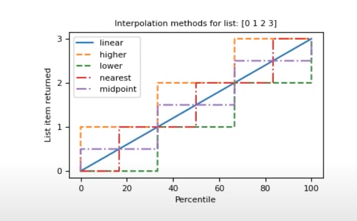
#In[]
a1 = np.array([0,1,2,3])
print(a1)
print(np.percentile(a1, [0,20,40,60,80,100], interpolation= 'linear'))
print(np.percentile(a1, [0,20,40,60,80,100], interpolation= 'higher'))
print(np.percentile(a1, [0,20,40,60,80,100], interpolation= 'lower'))
print(np.percentile(a1, [0,20,40,60,80,100], interpolation= 'nearest'))
print(np.percentile(a1, [0,20,40,60,80,100], interpolation= 'midpoint'))

#Out[]
[0 1 2 3]
[0.  0.6 1.2 1.8 2.4 3. ]
[0 1 2 2 3 3]
[0 0 1 1 2 3]
[0 1 1 2 2 3]
[0.  0.5 1.5 1.5 2.5 3. ]

any()

#In[]
a2 = np.array([[False, False, False],
              [False, True, True],
              [False, True, True]])
print(a2)
print(np.any(a2))
print(np.any(a2, axis=0))
print(np.any(a2, axis=1))

#한개라도 True가 있다면 True
#모두 False여야 False

#Out[]
[[False False False]
 [False  True  True]
 [False  True  True]]
 
True

[False  True  True]

[False  True  True]

all()

#In[]
a2 = np.array([[False, False, True],
              [True, True, True],
              [False, True, True]])
print(a2)
print(np.all(a2))
print(np.all(a2, axis=0))
print(np.all(a2, axis=1))

#모두 True여야 True
#한개라도 False가 있다 False

#Out[]
[[False False  True]
 [ True  True  True]
 [False  True  True]]
 
False

[False False  True]

[False  True False]

1:55:36

비교 연산(Comparison Operators)

#In[]


#Out[]

#In[]


#Out[]

#In[]


#Out[]

#In[]


#Out[]

### 2021.12.18

배열 전치 및 축 변경

#In[]
import numpy as np

a2 = np.array([[1,2,3,], [4,5,6], [7,8,9]])

print(a2)
print(a2.T)

#Out[]
[[1 2 3]
 [4 5 6]
 [7 8 9]]

[[1 4 7]
 [2 5 8]
 [3 6 9]]

#In[]
a3 = np.array([[[1,2,3], [4,5,6], [7,8,9]],
               [[1,2,3], [4,5,6], [7,8,9]],
               [[1,2,3], [4,5,6], [7,8,9]]])

print(a3)
print(a3.T)

#Out[]
[[[1 2 3]
  [4 5 6]
  [7 8 9]]

 [[1 2 3]
  [4 5 6]
  [7 8 9]]

 [[1 2 3]
  [4 5 6]
  [7 8 9]]]
----------------------
[[[1 1 1]
  [4 4 4]
  [7 7 7]]

 [[2 2 2]
  [5 5 5]
  [8 8 8]]

 [[3 3 3]
  [6 6 6]
  [9 9 9]]]

#In[]
print(a2)
print(a2.swapaxes(1,0))

#Out[]
[[1 2 3]
 [4 5 6]
 [7 8 9]]

[[1 4 7]
 [2 5 8]
 [3 6 9]]

#In[]
print(a3)
print(a3.swapaxes(0,1))       #0차원 축과 1차원 축을 바꿔라
print(a3.swapaxes(1,2))       #1차원 축과 2차원 축을 바꿔라

#Out[]
[[[1 2 3]
  [4 5 6]
  [7 8 9]]

 [[1 2 3]
  [4 5 6]
  [7 8 9]]

 [[1 2 3]
  [4 5 6]
  [7 8 9]]]
-------------------
[[[1 2 3]
  [1 2 3]
  [1 2 3]]

 [[4 5 6]
  [4 5 6]
  [4 5 6]]

 [[7 8 9]
  [7 8 9]
  [7 8 9]]]
------------------
[[[1 4 7]
  [2 5 8]
  [3 6 9]]

 [[1 4 7]
  [2 5 8]
  [3 6 9]]

 [[1 4 7]
  [2 5 8]
  [3 6 9]]]

배열 재구조화

• reshape(): 배열의 형상을 변경

#In[]
n1 = np.arange(1, 10)
print(n1)
print(n1.reshape(3,3))

#Out[]
[1 2 3 4 5 6 7 8 9]

[[1 2 3]
 [4 5 6]
 [7 8 9]]

• newaxis(): 새로운 축 추가

#In[1]
print(n1)
#Out[1]
[1 2 3 4 5 6 7 8 9]


#In[2]
print(n1[np.newaxis, :5])
#Out[2]
[[1 2 3 4 5]]


#In[3]
print(n1[:5, np.newaxis])
#Out[3]
[[1]
 [2]
 [3]
 [4]
 [5]]

배열 크기 변경 resize()

• 배열 모양만 변경

#In[1]
n2 = np.random.randint(0, 10, (2,5))
print(n2)
#Out[1]
[[4 4 8 0 7]
 [1 1 3 8 9]]

#In[2]
n2.resize((5,2))
print(n2)
#Out[2]
[[4 4]
 [8 0]
 [7 1]
 [1 3]
 [8 9]]

• 배열 크기 증가
• 남은 공간은 0으로 채워짐

#In[]
n2.resize((5,5))
print(n2)

#Out[]
[[7 1 6 8 1]
 [1 8 7 4 3]
 [0 0 0 0 0]
 [0 0 0 0 0]
 [0 0 0 0 0]]
 
 #코랩에서 실행이 안되어서 주피터노트북에서 실행!(값이 달라졌음)

• 배열 크기 감소
• 포함되지 않은 값은 삭제됨

#In[]
n2.resize((3,3))
print(n2)

#Out[]
[[7 1 6]
 [8 1 1]
 [8 7 4]]

배열 추가

• append(): 배열의 끝에 값 추가

#In[]
a2 = np.arange(1, 10).reshape(3,3)
print(a2)
b2 = np.arange(10,19).reshape(3,3)
print(b2)

#Out[]
[[1 2 3]
 [4 5 6]
 [7 8 9]]
 
[[10 11 12]
 [13 14 15]
 [16 17 18]]

• axis 지정이 없으면 1차원 배열 형태로 변형되어 결합

#In[]
c2 = np.append(a2, b2)
print(c2)

#Out[]
[ 1  2  3  4  5  6  7  8  9 10 11 12 13 14 15 16 17 18]

• axis를 0으로 지정
• shape[0]을 제외한 나머지 shape은 같아야 함

#In[]
c2 = np.append(a2, b2, axis = 0)
print(c2)

#Out[]
[[ 1  2  3]
 [ 4  5  6]
 [ 7  8  9]
 [10 11 12]
 [13 14 15]
 [16 17 18]]

• axis를 1로 지정
• shape[1]을 제외한 나머지 shape은 같아야 함

#In[]
c2 = np.append(a2, b2, axis = 1)
print(c2)

#Out[]
[[ 1  2  3 10 11 12]
 [ 4  5  6 13 14 15]
 [ 7  8  9 16 17 18]]

배열 연결

• concatenate(): 튜플이나 배열의 리스트를 인수로 사용해 배열 연결

#In[1]
a1 = np.array([1,3,5])
b1 = np.array([2,4,6])
np.concatenate([a1,b1])

#Out[1]
array([1, 3, 5, 2, 4, 6])

#In[2]
c1 = np.array([7,8,9])
np.concatenate([a1,b1,c1])

#Out[2]
array([1, 3, 5, 2, 4, 6, 7, 8, 9])

#In[1]
a2 = np.array([[1,2,3,],
               [4,5,6]])
np.concatenate([a2,a2])
#Out[1]
array([[1, 2, 3],
       [4, 5, 6],
       [1, 2, 3],
       [4, 5, 6]])
       
#In[2]
np.concatenate([a2,a2],axis=1)
#Out[2]
array([[1, 2, 3, 1, 2, 3],
       [4, 5, 6, 4, 5, 6]])

• vstack(): 수직 스택(vertical stack), 1차원으로 연결

#In[]
np.vstack([a2,a2])

#Out[]
array([[1, 2, 3],
       [4, 5, 6],
       [1, 2, 3],
       [4, 5, 6]])

• hstack(): 수평 스택(horizontal stack), 2차원으로 연결

#In[]
np.hstack([a2,a2])

#Out[]
array([[1, 2, 3, 1, 2, 3],
       [4, 5, 6, 4, 5, 6]])

• dstack(): 깊이 스택(depth stack), 3차원으로 연결

#In[]
np.dstack([a2,a2])

#Out[]
array([[[1, 1],
        [2, 2],
        [3, 3]],

       [[4, 4],
        [5, 5],
        [6, 6]]])

• stack(): 새로운 차원으로 연결

#In[]
np.stack([a2,a2])

#Out[]
array([[[1, 2, 3],
        [4, 5, 6]],

       [[1, 2, 3],
        [4, 5, 6]]])

배열 분할

• split(): 배열 분할

#In[1]
a1 = np.arange(0,10)
print(a1)
#Out[1]
[0 1 2 3 4 5 6 7 8 9]

#In[2]
b1, c1 = np.split(a1,[5])
print(b1, c1)
#Out[2]
[0 1 2 3 4] [5 6 7 8 9]

#In[3]
np.split(a1, [2,4,6,8])
#Out[3]
[array([0, 1]), array([2, 3]), array([4, 5]), array([6, 7]), array([8, 9])]

• vsplit(): 수직 분할, 1차원으로 분할

#In[]
a2 = np.arange(1, 10).reshape(3,3)
print(a2)

b2, c2 = np.vsplit(a2, [2])
print(b2)
print(c2)

#Out[]
[[1 2 3]
 [4 5 6]
 [7 8 9]]
 
[[1 2 3]
 [4 5 6]]
 
[[7 8 9]]

• hsplit(): 수평 분할, 2차원으로 분할

#In[]
a2 = np.arange(1, 10).reshape(3,3)
print(a2)

b2, c2 = np.hsplit(a2, [2])

print(b2)
print(c2)

#Out[]
[[1 2 3]
 [4 5 6]
 [7 8 9]]
 
[[1 2]
 [4 5]
 [7 8]]
 
[[3]
 [6]
 [9]]

• dsplit(): 깊이 분할, 3차원으로 분할

#In[]
a3 = np.arange(1, 28).reshape(3,3,3)
print(a3)

b3, c3 = np.dsplit(a3, [2])

print(b3)
print(c3)

#Out[]
[[[ 1  2  3]
  [ 4  5  6]
  [ 7  8  9]]

 [[10 11 12]
  [13 14 15]
  [16 17 18]]

 [[19 20 21]
  [22 23 24]
  [25 26 27]]]
--------------------
[[[ 1  2]
  [ 4  5]
  [ 7  8]]

 [[10 11]
  [13 14]
  [16 17]]

 [[19 20]
  [22 23]
  [25 26]]]
-----------------
[[[ 3]
  [ 6]
  [ 9]]

 [[12]
  [15]
  [18]]

 [[21]
  [24]
  [27]]]

### 2021.12.18

배열 값 삽입

• insert(): 배열의 특정 위치에 값 삽입
• axis를 지정하지 않으면 1차원 배열로 변환
• 추가할 방향을 axis로 지정
• 원본 배열 변경없이 새로운 배열 반환

#In[1]
import numpy as np
a1 = np.array([1,2,3,4,5])
 
print(a1)
b1 = np.insert(a1, 0, 10)    # a1의 0번째에 10을 넣어라!
print(b1)

#Out[1]
[1 2 3 4 5]
[10  1  2  3  4  5]

#In[2]
print(a1)
#Out[2]
[1 2 3 4 5]      #a1의 값은 변하지 않는다!

#In[3]
c1 = np.insert(a1, 2, 10)
print(c1)
#Out[3]
[ 1  2 10  3  4  5]

#In[1]
a2 = np.array([[1,2,3,], [4,5,6], [7,8,9]])
print(a2)
#Out[1]
[[1 2 3]
 [4 5 6]
 [7 8 9]]

#In[2]
b2 = np.insert(a2, 1, 10, axis=0)
print(b2)
#Out[2]
[[ 1  2  3]
 [10 10 10]
 [ 4  5  6]
 [ 7  8  9]]

#In[3]
c2 =np.insert(a2, 1, 10, axis=1)
print(c2)
#Out[3]
[[ 1 10  2  3]
 [ 4 10  5  6]
 [ 7 10  8  9]]

배열 값 수정

• 배열의 인덱싱으로 접근하여 값 수정

#In[]
print(a1)
a1[0] = 6
a1[1] = 7
print(a1)

#Out[]
[1 2 3 4 5]
[6 7 3 4 5]

#In[1]
a1[0:1] = 9
print(a1)
#Out[1]
[9 7 3 4 5]

#In[2]
i = np.array([1,3,4])
a1[i] = 0
print(a1)
#Out[2]
[9 0 3 0 0]

#In[3]
a1[i] += 4
print(a1)
#Out[3]
[9 4 3 4 4]

#In[]
print(a2)
a2[1, 1] = 1
a2[2, 2] = 2
a2[0] = 1
print(a2)

#Out[]
[[1 2 3]
 [4 5 6]
 [7 8 9]]
[[1 1 1]
 [4 1 6]
 [7 8 2]]

#In[1]
a2[1:, 2] = 9
print(a2)

#Out[1]
[[1 1 1]
 [4 1 9]
 [7 8 9]]

#In[2]
row = np.array([0,1])
col = np.array([1,2])
a2[row,col] = 0
print(a2)

#Out[2]
[[1 0 1]
 [4 1 0]
 [7 8 9]]

배열 값 삭제

• delete(): 배열의 특정 위치에 값 삭제
• axis를 지정하지 않으면 1차원 배열로 변환
• 삭제할 방향을 axis로 지정
• 원본 배열 변경없이 새로운 배열 반환

#In[]
print(a1)
b1 = np.delete(a1, 1)
print(b1)

#Out[]
[9 4 3 4 4]
[9 3 4 4]

#In[1]
print(a2)
#Out[1]
[[1 0 1]
 [4 1 0]
 [7 8 9]]

#In[2]
b2 = np.delete(a2, 1, axis=0)
print(b2)
#Out[2]
[[1 0 1]
 [7 8 9]]

#In[3]
c2 = np.delete(a2, 1, axis=1)
print(c2)
#Out[3]
[[1 1]
 [4 0]
 [7 9]]

배열 복사

• 리스트 자료형과 달리 배열의 슬라이스는 복사본이 아님

#In[1]
print(a2)
#Out[1]
[[1 0 1]
 [4 0 0]
 [7 8 9]]

#In[2]
a2_sub = a2[:2, :2]
print(a2_sub)
#Out[2]
[[1 0]
 [4 0]]

#In[3]
a2_sub[:, 1] = 2
print(a2_sub)
#Out[3]
[[1 2]
 [4 2]]

#In[4]
print(a2)
#Out[4]
[[1 2 1]
 [4 2 0]
 [7 8 9]]
 
 #넘파이는 슬라이싱한 값이 변경되면 원본값도 변경된다.

• copy(): 배열이나 하위 배열 내의 값을 명시적으로 복사

#In[1]
print(a2)
#Out[1]
[[1 2 1]
 [4 2 0]
 [7 8 9]]
 
#In[2]
a2_sub_copy = a2[:2, :2].copy()
print(a2_sub_copy)
#Out[2]
[[1 2]
 [4 2]]

#In[3]
a2_sub_copy[:, 1] = 0
print(a2_sub_copy)
#Out[3]
[[1 0]
 [4 0]]

#In[4]
print(a2)
#Out[4]
[[1 2 1]
 [4 2 0]
 [7 8 9]]
 
 #copy()를 통해서 복사하면 원본은 변경이 되지 않는다.

### 2021.12.17

MNIST 손글씨 이미지 데이터셋

MNIST 데이터셋은 위 그림과 같이 0에서 9까지 10가지로 분류될 수 있는 손글씨 숫자 이미지 70,000개로 이루어져 있습니다.

각 이미지는 28×28 픽셀로 구성되고 각 픽셀은 아래와 같이 0~255 사이의 숫자 행렬로 표현됩니다.

이러한 60,000개의 이미지는 인공 신경망의 훈련 (Training)에 사용되고, 10,000개의 이미지는 테스트 (Test)에 사용됩니다.

이번 페이지에서는 Dense 층들로 구성되는 완전 연결된 인공신경망 (Fully-Connected Neural Network)을 이용해서 MNIST 데이터셋을 분류해 보겠습니다.

예제

import tensorflow as tf

# 1. MNIST 데이터셋 임포트
mnist = tf.keras.datasets.mnist
(x_train, y_train), (x_test, y_test) = mnist.load_data()

# 2. 데이터 전처리
x_train, x_test = x_train/255.0, x_test/255.0

# 3. 모델 구성
model = tf.keras.models.Sequential([
    tf.keras.layers.Flatten(input_shape=(28, 28)),
    tf.keras.layers.Dense(512, activation=tf.nn.relu),
    tf.keras.layers.Dense(10, activation=tf.nn.softmax)
])

# 4. 모델 컴파일
model.compile(optimizer='adam',
              loss='sparse_categorical_crossentropy',
              metrics=['accuracy'])

# 5. 모델 훈련
model.fit(x_train, y_train, epochs=5)

# 6. 정확도 평가
test_loss, test_acc = model.evaluate(x_test, y_test)
print('테스트 정확도:', test_acc)

model.save('my_model1.h5')

#Out[]
Epoch 1/5
1875/1875 [==============================] - 7s 4ms/step - loss: 0.2026 - accuracy: 0.9408
Epoch 2/5
1875/1875 [==============================] - 8s 4ms/step - loss: 0.0808 - accuracy: 0.9753
Epoch 3/5
1875/1875 [==============================] - 7s 4ms/step - loss: 0.0514 - accuracy: 0.9837
Epoch 4/5
1875/1875 [==============================] - 7s 4ms/step - loss: 0.0376 - accuracy: 0.9880
Epoch 5/5
1875/1875 [==============================] - 7s 4ms/step - loss: 0.0266 - accuracy: 0.9916
313/313 [==============================] - 1s 2ms/step - loss: 0.0643 - accuracy: 0.9811
테스트 정확도: 0.9811000227928162

설명

0. tensorflow 불러오기

#tensorflow 라이브러리를 불러옵니다.
import tensorflow as tf

1. MNIST 데이터셋 임포트

mnist = tf.keras.datasets.mnist
(x_train, y_train), (x_test, y_test) = mnist.load_data()

tensorflow에서 직접 MNIST 손글씨 이미지 데이터셋을 불러와서 사용합니다.

load_data() 함수는 x_train, y_train, x_test, y_test 네 개의 NumPy 어레이를 반환합니다.

x_train, x_test는 28×28 픽셀의 각 손글씨 이미지 데이터이고, y_train, y_test는 분류에 사용되는 0~9 사이의 레이블 값을 갖습니다.

#In[1]
print("x_train 데이터 형태 :", x_train.shape)
print("x_train[0] 데이터 형태 :", x_train[0].shape)
print("y_train 데이터 형태 :", y_train.shape)

#Out[1]
x_train 데이터 형태 : (60000, 28, 28)
x_train[0] 데이터 형태 : (28, 28)
y_train 데이터 형태 : (60000,)

#In[2]
num = x_train[0]
for i in range(28):
    for j in range(28):
         print("{:4d}".format(num[i][j]), end="")
    print()

#Out[2]

이러한 60,000개의 이미지는 인공 신경망의 훈련 (Training)에 사용되고, 10,000개의 이미지는 테스트 (Test)에 사용됩니다.

이번 페이지에서는 Dense 층들로 구성되는 완전 연결된 인공신경망 (Fully-Connected Neural Network)을 이용해서 MNIST 데이터셋을 분류해 보겠습니다.

2.  데이터 전처리

# 0 ~ 255.0 사이의 값을 갖는 픽셀값들을 0~1.0 사이의 값을 갖도록 변환합니다.

x_train, x_test = x_train/255.0, x_test/255.0

3.  모델 구성

model = tf.keras.models.Sequential([
    tf.keras.layers.Flatten(input_shape=(28, 28)),
    tf.keras.layers.Dense(512, activation=tf.nn.relu),
    tf.keras.layers.Dense(10, activation=tf.nn.softmax)
])

tf.keras.models.Sequential()을 이용해서 인공신경망 모델을 구성합니다.

입력층 (Input layer)에서 Flatten()을 이용해서 28×28 픽셀의 값을 784개의 1차원 배열로 변환합니다.

다음 두 개의 뉴런 층 (Neuron layer)은 Dense()를 이용해서 완전 연결된 층 (Fully-connected layer)를 구성합니다.

각 층은 512개와 10개의 인공 뉴런 노드를 갖고 활성화 함수 (activation function)로는 각각 ReLU (tf.nn.relu)와 소프트맥스 (tf.nn.softmax)를 사용합니다.

4.  모델 컴파일

model.compile(optimizer='adam',
              loss='sparse_categorical_crossentropy',
              metrics=['accuracy'])

다음은 모델 컴파일 단계입니다. 학습 과정에서 손실 함수 (Loss function)를 줄이기 위해 사용되는 optimizer로는 Adam (Adaptive Momentum estimation)을 사용합니다.

손실 함수는 ‘sparse_categorical_crossentropy’를 지정하고, 평가 지표로는 정확도 (accuracy)를 사용합니다.

정확도는 테스트 이미지 중 올바르게 분류한 비율을 의미합니다.

5. 모델 훈련

#In[]
model.fit(x_train, y_train, epochs=5)

#Out[]
Epoch 1/5
1875/1875 [==============================] - 10s 5ms/step - loss: 0.1985 - accuracy: 0.9413
Epoch 2/5
1875/1875 [==============================] - 9s 5ms/step - loss: 0.0806 - accuracy: 0.9743
Epoch 3/5
1875/1875 [==============================] - 9s 5ms/step - loss: 0.0526 - accuracy: 0.9835
Epoch 4/5
1875/1875 [==============================] - 9s 5ms/step - loss: 0.0373 - accuracy: 0.9881
Epoch 5/5
1875/1875 [==============================] - 9s 5ms/step - loss: 0.0275 - accuracy: 0.9911
<tensorflow.python.keras.callbacks.History at 0x7fcb10ae1d90>

학습 과정은 위와 같이 이루어지며, 학습 데이터에 대한 정확도가 출력됩니다.

model.fit() 메서드에 학습 데이터와, 레이블, 에포크를 순서대로 입력하면, 학습이 이루어집니다.

에포크(epoch)는 60,000개의 전체 학습 데이터를 몇 번 반복해서 학습할지를 의미합니다.

model.save('my_model2.h5')

6. 정확도 평가

#In[]
test_loss, test_acc = model.evaluate(x_test, y_test)
print('테스트 정확도:', test_acc)

#Out[]
313/313 [==============================] - 1s 3ms/step - loss: 0.0707 - accuracy: 0.9785
테스트 정확도: 0.9785000085830688

결과는 위와 같습니다. 

model.evaluate()를 이용해서 10,000개의 테스트 샘플에 대해 손실 (loss)과 정확도 (accuracy)를 평가합니다.

간단한 인공신경망과 다섯 번 에포크의 학습만으로 98.02%의 정확도로 MNIST 이미지를 분류할 수 있음을 알 수 있습니다.

Matplotlib을 이용해서 에포크에 따른 정확도 (accuracy)와 손실 (loss) 값을 확인할 수 있습니다.

#In[]
loss, accuracy = [], []
for i in range(10):
    model.fit(x_train, y_train, epochs=1)
    loss.append(model.evaluate(x_test, y_test)[0])
    accuracy.append(model.evaluate(x_test, y_test)[1])

print(accuracy)

#Out[]
1875/1875 [==============================] - 9s 5ms/step - loss: 0.0202 - accuracy: 0.9933
313/313 [==============================] - 1s 2ms/step - loss: 0.0603 - accuracy: 0.9814
313/313 [==============================] - 1s 2ms/step - loss: 0.0603 - accuracy: 0.9814
1875/1875 [==============================] - 8s 4ms/step - loss: 0.0168 - accuracy: 0.9942
313/313 [==============================] - 1s 2ms/step - loss: 0.0819 - accuracy: 0.9775
313/313 [==============================] - 1s 2ms/step - loss: 0.0819 - accuracy: 0.9775
1875/1875 [==============================] - 8s 4ms/step - loss: 0.0148 - accuracy: 0.9950
313/313 [==============================] - 1s 3ms/step - loss: 0.0738 - accuracy: 0.9806
313/313 [==============================] - 1s 3ms/step - loss: 0.0738 - accuracy: 0.9806
1875/1875 [==============================] - 9s 5ms/step - loss: 0.0134 - accuracy: 0.9955
313/313 [==============================] - 1s 3ms/step - loss: 0.0662 - accuracy: 0.9833
313/313 [==============================] - 1s 2ms/step - loss: 0.0662 - accuracy: 0.9833
1875/1875 [==============================] - 8s 4ms/step - loss: 0.0101 - accuracy: 0.9965
313/313 [==============================] - 1s 2ms/step - loss: 0.0771 - accuracy: 0.9820
313/313 [==============================] - 1s 2ms/step - loss: 0.0771 - accuracy: 0.9820
1875/1875 [==============================] - 8s 4ms/step - loss: 0.0112 - accuracy: 0.9964
313/313 [==============================] - 1s 2ms/step - loss: 0.0744 - accuracy: 0.9821
313/313 [==============================] - 1s 2ms/step - loss: 0.0744 - accuracy: 0.9821
1875/1875 [==============================] - 8s 4ms/step - loss: 0.0075 - accuracy: 0.9974
313/313 [==============================] - 1s 2ms/step - loss: 0.0820 - accuracy: 0.9828
313/313 [==============================] - 1s 2ms/step - loss: 0.0820 - accuracy: 0.9828
1875/1875 [==============================] - 8s 4ms/step - loss: 0.0104 - accuracy: 0.9968
313/313 [==============================] - 1s 3ms/step - loss: 0.1053 - accuracy: 0.9808
313/313 [==============================] - 1s 2ms/step - loss: 0.1053 - accuracy: 0.9808
1875/1875 [==============================] - 10s 5ms/step - loss: 0.0066 - accuracy: 0.9979
313/313 [==============================] - 1s 2ms/step - loss: 0.0901 - accuracy: 0.9814
313/313 [==============================] - 1s 2ms/step - loss: 0.0901 - accuracy: 0.9814
1875/1875 [==============================] - 9s 5ms/step - loss: 0.0084 - accuracy: 0.9975
313/313 [==============================] - 1s 3ms/step - loss: 0.0798 - accuracy: 0.9840
313/313 [==============================] - 1s 2ms/step - loss: 0.0798 - accuracy: 0.9840
[0.9814000129699707, 0.9775000214576721, 0.9805999994277954, 0.983299970626831, 0.9819999933242798, 0.9821000099182129, 0.9828000068664551, 0.9807999730110168, 0.9814000129699707, 0.984000027179718]

1회의 에포크마다 model.evaluate()의 loss, accuracy 값을 저장합니다.

결과는 아래와 같습니다.

model.save('my_model3.h5')

## Ex 10-6. MNIST 손글씨 인식 프로그램.

import sys
from PyQt5.QtWidgets import *
from PyQt5.QtGui import *
from PyQt5.QtCore import *
import numpy as np
import tensorflow as tf


class MyApp(QMainWindow):

    def __init__(self):
        super().__init__()
        self.image = QImage(QSize(400, 400), QImage.Format_RGB32)
        self.image.fill(Qt.white)
        self.drawing = False
        self.brush_size = 30
        self.brush_color = Qt.black
        self.last_point = QPoint()
        self.loaded_model = None
        self.initUI()

    def initUI(self):
        menubar = self.menuBar()
        menubar.setNativeMenuBar(False)
        filemenu = menubar.addMenu('File')

        load_model_action = QAction('Load model', self)
        load_model_action.setShortcut('Ctrl+L')
        load_model_action.triggered.connect(self.load_model)

        save_action = QAction('Save', self)
        save_action.setShortcut('Ctrl+S')
        save_action.triggered.connect(self.save)

        clear_action = QAction('Clear', self)
        clear_action.setShortcut('Ctrl+C')
        clear_action.triggered.connect(self.clear)

        filemenu.addAction(load_model_action)
        filemenu.addAction(save_action)
        filemenu.addAction(clear_action)

        self.statusbar = self.statusBar()

        self.setWindowTitle('MNIST Classifier')
        self.setGeometry(300, 300, 400, 400)
        self.show()

    def paintEvent(self, e):
        canvas = QPainter(self)
        canvas.drawImage(self.rect(), self.image, self.image.rect())

    def mousePressEvent(self, e):
        if e.button() == Qt.LeftButton:
            self.drawing = True
            self.last_point = e.pos()

    def mouseMoveEvent(self, e):
        if (e.buttons() & Qt.LeftButton) & self.drawing:
            painter = QPainter(self.image)
            painter.setPen(QPen(self.brush_color, self.brush_size, Qt.SolidLine, Qt.RoundCap))
            painter.drawLine(self.last_point, e.pos())
            self.last_point = e.pos()
            self.update()

    def mouseReleaseEvent(self, e):
        if e.button() == Qt.LeftButton:
            self.drawing = False

            arr = np.zeros((28, 28))
            for i in range(28):
                for j in range(28):
                    arr[j, i] = 1 - self.image.scaled(28, 28).pixelColor(i, j).getRgb()[0] / 255.0
            arr = arr.reshape(-1, 28, 28)

            if self.loaded_model:
                pred = self.loaded_model.predict(arr)[0]
                pred_num = str(np.argmax(pred))
                self.statusbar.showMessage('숫자 ' + pred_num + '입니다.')

    def load_model(self):
        fname, _ = QFileDialog.getOpenFileName(self, 'Load Model', '')

        if fname:
            self.loaded_model = tf.keras.models.load_model(fname)
            self.statusbar.showMessage('Model loaded.')

    def save(self):
        fpath, _ = QFileDialog.getSaveFileName(self, 'Save Image', '', "PNG(*.png);;JPEG(*.jpg *.jpeg);;All Files(*.*) ")

        if fpath:
            self.image.scaled(28, 28).save(fpath)

    def clear(self):
        self.image.fill(Qt.white)
        self.update()
        self.statusbar.clearMessage()

if __name__ == '__main__':
    app = QApplication(sys.argv)
    ex = MyApp()
    sys.exit(app.exec_())

### 2021.12.17

이전 페이지에서 각 뉴런층의 이름, 자료형, 활성화함수와 같은 다양한 정보를 확인하는 방법에 대해 알아보았습니다.

이 페이지에서는 특정 입력 데이터에 대해 각 뉴런층이 출력하는 값을 확인하는 방법에 대해 소개합니다.

훈련 데이터 준비하기

import tensorflow as tf
import numpy as np

tf.random.set_seed(0)


# 1. 훈련 데이터 준비하기
x_train = np.array([[1, 0, 0], [0, 1, 0], [0, 0, 1]])
y_train = np.array([[0], [1], [1]])

우선 tf.random 모듈의 set_seed() 함수를 사용해서 랜덤 시드를 설정했습니다.

예제에서 x_train, y_train은 각각 훈련에 사용할 입력값, 출력값입니다.

이 페이지에서는 훈련은 진행하지 않고 입력 데이터 (x_train)에 대해 각 뉴런층이 출력하는 값을 확인합니다.

뉴런층 만들기

# 2. 뉴런층 만들기
input_layer = tf.keras.layers.InputLayer(input_shape=(3,))
hidden_layer = tf.keras.layers.Dense(units=4, activation='relu')
output_layer = tf.keras.layers.Dense(units=2, activation='softmax')

아래와 같은 간단한 신경망 모델을 구성하기 위한 뉴런층을 각각 만들었습니다.

길이 3을 갖는 벡터 입력을 받고, 은닉층은 네 개의 뉴런 노드를 가지며, 출력층은 두 개의 뉴런 노드를 가집니다.

은닉층의 활성화함수는 ‘relu’, 출력층의 활성화함수는 ‘softmax’로 지정했습니다.

Neural Network 구성하기

# 3. 모델 구성하기
model = tf.keras.Sequential([
  input_layer,
  hidden_layer,
  output_layer
  ])

tf.keras 모듈의 Sequantial 클래스는 Neural Network의 각 층을 순서대로 쌓을 수 있도록 합니다.

앞에서 만든 뉴런층을 순서대로 입력해서 신경망 모델을 구성합니다.

Neural Network 컴파일하기

# 4. 모델 컴파일하기
model.compile(loss='mse', optimizer='Adam')

손실 함수로 ‘mse’를, 옵티마이저로 ‘Adam’을 지정했습니다.

이 페이지의 예제에서는 훈련을 진행하지 않기 때문에 컴파일 과정은 생략할 수 있습니다.

은닉층의 출력값 확인하기

# 5. 은닉층의 출력 확인하기
intermediate_layer_model = tf.keras.Model(inputs=model.input, outputs=model.layers[0].output)
intermediate_output = intermediate_layer_model(x_train)

print('======== Inputs ========')
print(x_train)

print('\n======== Weights of Hidden Layer ========')
print(hidden_layer.get_weights()[0])

print('\n======== Outputs of Hidden Layer ========')
print(intermediate_output)

#Out[]
======== Inputs ========
[[1 0 0]
 [0 1 0]
 [0 0 1]]

======== Weights of Hidden Layer ========
[[-0.3851872  -0.54333335  0.0655309   0.1134268 ]
 [-0.15428883  0.5699866  -0.01254469  0.9223561 ]
 [ 0.36428273 -0.6936733   0.38850498  0.30073535]]

======== Outputs of Hidden Layer ========
tf.Tensor(
[[0.         0.         0.0655309  0.1134268 ]
 [0.         0.5699866  0.         0.9223561 ]
 [0.36428273 0.         0.38850498 0.30073535]], shape=(3, 4), dtype=float32)

tf.keras 모듈의 Model 클래스를 사용해서 새로운 모델 (intermediate_layer_model)을 하나 만들었습니다.

이 모델은 앞에서 구성한 전체 모델의 입력을 입력으로 하고,

첫번째 뉴런층 (hidden_layer)의 출력을 출력으로 하는 신경망 모델입니다.

이 모델에 훈련 데이터 (x_train)을 입력하면 첫번째 뉴런층의 출력을 반환합니다.

첫번째 뉴런층, 즉 은닉층의 출력은 아래와 같이 계산됩니다.

우선 입력 데이터 [1, 0, 0]에 대해 은닉층의 시냅스 가중치가 곱해집니다.

즉, 입력층 첫번째 노드의 입력 1에 시냅스 가중치 [-0.3851872 -0.54333335 0.0655309 0.1134268 ]가 곱해집니다.

다음으로 은닉층의 활성화함수인 ReLU (Rectified Linear Unit)가 적용되어서

0보다 작은 값은 0이되고, 0보다 큰 값은 그대로 출력값이 됩니다.

출력층의 출력값 확인하기

# 6. 출력층의 출력 확인하기
pred = model.predict(x_train)

print('\n======== Outputs of Output Layer ========')
print(pred)

#Out[]
======== Outputs of Output Layer ========
[[0.45516008 0.5448399 ]
 [0.18469977 0.8153002 ]
 [0.4541021  0.5458979 ]]

전체 신경망의 출력값은 Model 클래스의 predict() 메서드를 사용해서 간단하게 얻을 수 있습니다.

세 개의 값을 갖는 세 개의 입력 데이터 벡터에 대해 두 개의 값을 갖는 벡터 세 개를 출력합니다.

전체 예제 코드

import tensorflow as tf
import numpy as np

tf.random.set_seed(0)


# 1. 훈련 데이터 준비하기
x_train = np.array([[1, 0, 0], [0, 1, 0], [0, 0, 1]])
y_train = np.array([[0], [1], [1]])


# 2. 뉴런층 만들기
input_layer = tf.keras.layers.InputLayer(input_shape=(3,))
hidden_layer = tf.keras.layers.Dense(units=4, activation='relu')
output_layer = tf.keras.layers.Dense(units=2, activation='softmax')


# 3. 모델 구성하기
model = tf.keras.Sequential([
  input_layer,
  hidden_layer,
  output_layer
  ])

# 4. 모델 컴파일하기
model.compile(loss='mse', optimizer='Adam')


# 5. 은닉층의 출력 확인하기
intermediate_layer_model = tf.keras.Model(inputs=model.input, outputs=model.layers[0].output)
intermediate_output = intermediate_layer_model(x_train)

print('======== Inputs ========')
print(x_train)

print('\n======== Weights of Hidden Layer ========')
print(hidden_layer.get_weights()[0])

print('\n======== Outputs of Hidden Layer ========')
print(intermediate_output)

# 6. 출력층의 출력 확인하기
pred = model.predict(x_train)

print('\n======== Outputs of Output Layer ========')
print(pred)

#Out[]
======== Inputs ========
[[1 0 0]
 [0 1 0]
 [0 0 1]]

======== Weights of Hidden Layer ========
[[-0.3851872  -0.54333335  0.0655309   0.1134268 ]
 [-0.15428883  0.5699866  -0.01254469  0.9223561 ]
 [ 0.36428273 -0.6936733   0.38850498  0.30073535]]

======== Outputs of Hidden Layer ========
tf.Tensor(
[[0.         0.         0.0655309  0.1134268 ]
 [0.         0.5699866  0.         0.9223561 ]
 [0.36428273 0.         0.38850498 0.30073535]], shape=(3, 4), dtype=float32)

======== Outputs of Output Layer ========
[[0.45516008 0.5448399 ]
 [0.18469977 0.8153002 ]
 [0.4541021  0.5458979 ]]

### 2021.12.17

tf.keras.layers.Layer는 Neural Network의 모든 레이어 객체가 상속하는 클래스입니다.

tf.keras.layers.Layer의 다양한 속성 (Attribute)을 이용해서 각 레이어에 대한 정보를 확인할 수 있습니다.

뉴런층의 이름(name)과 자료형 (dtype)

import tensorflow as tf

tf.random.set_seed(0)


# 1. 뉴런층 만들기
input_layer = tf.keras.layers.InputLayer(input_shape=(3,))
hidden_layer = tf.keras.layers.Dense(units=4, activation='relu')
output_layer = tf.keras.layers.Dense(units=2, activation='softmax')


# 2. 모델 구성하기
model = tf.keras.Sequential([
    input_layer,
    hidden_layer,
    output_layer
    ])


# 3. 모델 컴파일하기
model.compile(loss='mse', optimizer='Adam')


# 4. 뉴런층의 이름과 자료형
print(input_layer.name, input_layer.dtype)
print(hidden_layer.name, hidden_layer.dtype)
print(output_layer.name, output_layer.dtype)

#Out[]
input_1 float32
dense float32
dense_1 float32

print(model.layers[0].name)
print(model.layers[1].name)
print(model.layers[2].name)

#Out[]
dense
dense_1
---------------------------------------------------------------------------
IndexError                                Traceback (most recent call last)
/var/folders/xx/_99p48vj7pg7bs_kpl7838_00000gn/T/ipykernel_92980/147579868.py in <module>
      1 print(model.layers[0].name)
      2 print(model.layers[1].name)
----> 3 print(model.layers[2].name)

IndexError: list index out of range

model.layers는 구성한 Neural Network 모델의 (입력층을 제외한) 뉴런층 레이어 객체를 리스트의 형태로 반환합니다.

model.layers[0]은 모델의 첫번째 뉴런층, 즉 은닉층 (hidden layer)입니다.

model.layers[1]은 모델의 두번째 뉴런층, 즉 출력층 (output_layer)입니다.

모델이 (입력층을 제외한) 두 개의 뉴런층을 포함하기 때문에

model.layers[2].name을 출력하면 에러를 발생합니다.

뉴런층의 입력(input)과 출력(output)

print(input_layer.input)
print(input_layer.output)
print()

print(hidden_layer.input)
print(hidden_layer.output)
print()

print(hidden_layer.input.shape)
print(hidden_layer.output.shape)
print()

print(output_layer.input)
print(output_layer.output)

#Out[]
Tensor("input_1:0", shape=(None, 3), dtype=float32)
Tensor("input_1:0", shape=(None, 3), dtype=float32)

Tensor("input_1:0", shape=(None, 3), dtype=float32)
Tensor("dense/Relu:0", shape=(None, 4), dtype=float32)

(None, 3)
(None, 4)

Tensor("dense/Relu:0", shape=(None, 4), dtype=float32)
Tensor("dense_1/Softmax:0", shape=(None, 2), dtype=float32)

input은 뉴런층의 입력 텐서 (input tensor)입니다.

output은 뉴런층의 출력 텐서 (output tensor)입니다.

은닉층 (hidden_layer)의 입력과 출력의 형태 (shape)를 출력해보면

입력 텐서는 길이 3의 형태, 출력 텐서는 길이 4의 형태를 가짐을 알 수 있습니다.

예를 들어, (None, 3)은 길이 3의 벡터의 시퀀스형태가 될 수 있음을 의미합니다.

뉴런층의 활성화함수 (activation)

#In[]
print(hidden_layer.activation)
print(hidden_layer.activation.__name__)
print(output_layer.activation)
print(output_layer.activation.__name__)

#Out[]
<function relu at 0x7fceb66d0430>
relu
<function softmax at 0x7fceb66bdd30>
softmax

activation은 뉴런 노드의 활성화함수 (Activation function)를 나타냅니다.
"__Name"__"*을 사용해서 활성화함수의 이름을 출력했습니다.

뉴런층의 가중치 (weights)

#In[]
print(hidden_layer.weights)
print()
print(output_layer.weights)

#Out[]
[<tf.Variable 'dense/kernel:0' shape=(3, 4) dtype=float32, numpy=
array([[-0.3851872 , -0.54333335,  0.0655309 ,  0.1134268 ],
       [-0.15428883,  0.5699866 , -0.01254469,  0.9223561 ],
       [ 0.36428273, -0.6936733 ,  0.38850498,  0.30073535]],
      dtype=float32)>, <tf.Variable 'dense/bias:0' shape=(4,) dtype=float32, numpy=array([0., 0., 0., 0.], dtype=float32)>]

[<tf.Variable 'dense_1/kernel:0' shape=(4, 2) dtype=float32, numpy=
array([[ 0.11082816, -0.55741405],
       [ 0.7298498 ,  0.5545671 ],
       [ 0.29023337,  0.0607245 ],
       [-0.971118  ,  0.74701834]], dtype=float32)>, <tf.Variable 'dense_1/bias:0' shape=(2,) dtype=float32, numpy=array([0., 0.], dtype=float32)>]

weights를 사용해서 각 뉴런층의 시냅스 가중치에 대한 정보를 얻을 수 있습니다.

get_weights() 메세드

#In[]
print(hidden_layer.get_weights())
print()
print(output_layer.get_weights())

#Out[]
[array([[-0.3851872 , -0.54333335,  0.0655309 ,  0.1134268 ],
       [-0.15428883,  0.5699866 , -0.01254469,  0.9223561 ],
       [ 0.36428273, -0.6936733 ,  0.38850498,  0.30073535]],
      dtype=float32), array([0., 0., 0., 0.], dtype=float32)]

[array([[ 0.11082816, -0.55741405],
       [ 0.7298498 ,  0.5545671 ],
       [ 0.29023337,  0.0607245 ],
       [-0.971118  ,  0.74701834]], dtype=float32), array([0., 0.], dtype=float32)]

get_weights() 메서드를 사용하면 시냅스 가중치를 NumPy 어레이 형태로 얻을 수 있습니다.

### 2021.12.17

tf.constant

tf.constant 함수는 상수 텐서를 생성합니다.

예제 #1

tf.constant 함수는 파이썬 리스트 또는 NumPy 어레이로부터 상수 텐서를 생성합니다.

#In[]
import tensorflow as tf
import numpy as np

a = tf.constant([1, 2, 3, 4])
b = tf.constant(np.array([1, 2, 3, 4]))

print(a)
print(b)

#Out[]
tf.Tensor([1 2 3 4], shape=(4,), dtype=int32)
tf.Tensor([1 2 3 4], shape=(4,), dtype=int64)

예제 #2

tf.constant 함수의 dtype은 생성될 값의 자료형을 지정합니다.

shape을 지정하면 입력값을 지정한 형태로 생성합니다.

#In[]
import tensorflow as tf
import numpy as np

a = tf.constant([1, 2, 3, 4], dtype=tf.float64)
b = tf.constant(0, shape=(2, 3))

print(a)
print(b)

#Out[]
tf.Tensor([1. 2. 3. 4.], shape=(4,), dtype=float64)
tf.Tensor(
[[0 0 0]
 [0 0 0]], shape=(2, 3), dtype=int32)

tf. TenserShape

tf.TenseorShape은 텐서의 형태를 나타냅니다

예제 #1

#In[]
import tensorflow as tf
import numpy as np

a = tf.constant([1,2,3,4])
b = tf.constant(np.array([1,2,3,4]))
print(a)
print(b)

#Out[]
tf.Tensor([1 2 3 4], shape=(4,), dtype=int32)
tf.Tensor([1 2 3 4], shape=(4,), dtype=int64)

tf.constant 함수는 파이썬 리스트 또는 NumPy 어레이로부터 상수 텐서를 생성합니다.

예제 #2

#In[]
a = tf.constant([1,2,3,4], dtype=tf.float64)
b = tf.constant(0, shape=(2,3))

print(a)
print(b)

#Out[]
tf.Tensor([1. 2. 3. 4.], shape=(4,), dtype=float64)
tf.Tensor(
[[0 0 0]
 [0 0 0]], shape=(2, 3), dtype=int32)

tf.constant 함수의 dtype은 생성될 값의 자료형을 지정합니다.

shape을 지정하면 입력값을 지정한 형태로 생성합니다.

tf.rank

tf.rank 함수는 입력한 텐서의 rank를 반환합니다.

#In[]
scalar = tf.constant(1)
vector = tf.constant([1, 2, 3])
matrix = tf.constant([[1, 2, 3], [4, 5, 6], [7, 8, 9]])
tensor = tf.constant([[[1, 2, 3], [4, 5, 6], [7, 8, 9]],
                    [[1, 2, 3], [4, 5, 6], [7, 8, 9]],
                    [[1, 2, 3], [4, 5, 6], [7, 8, 9]]])

print(tf.rank(scalar))
print(tf.rank(vector))
print(tf.rank(matrix))
print(tf.rank(tensor))

#Out[]
tf.Tensor(0, shape=(), dtype=int32)
tf.Tensor(1, shape=(), dtype=int32)
tf.Tensor(2, shape=(), dtype=int32)
tf.Tensor(3, shape=(), dtype=int32)

텐서 (Tensor) 객체의 랭크 (Rank)는 차원의 수 (n-dimension)입니다.

tf.rank()는 텐서의 랭크를 반환합니다.

텐서 scalar, vector, matrix, tensor는 각각 랭크 0, 1, 2, 3를 가집니다.

tf.cast

tf.cast 함수는 텐서를 새로운 자료형으로 변환합니다.

예제 #1

#In[]
x = tf.constant([1.8,2.2], dtype=tf.float32)
y = tf.cast(x, tf.int32)

print(x)
print(y)

#Out[]
tf.Tensor([1.8 2.2], shape=(2,), dtype=float32)
tf.Tensor([1 2], shape=(2,), dtype=int32)

x는 (2,) 형태를 갖고, tf.float32 자료형을 갖는 텐서입니다.

tf.cast()를 사용해서 tf.int32 자료형을 갖도록 변환했습니다.

예제 #2

#In[]
x = tf.constant([1.8, 2.2], dtype=tf.float32)
y = tf.dtypes.cast(x, tf.int32)

print(x)
print(y)

#Out[]
tf.Tensor([1.8 2.2], shape=(2,), dtype=float32)
tf.Tensor([1 2], shape=(2,), dtype=int32)

tf.dtypes.cast()는 tf.cast()의 alias입니다.

tf.dtypes.cast()를 사용해서 tf.int32 자료형을 갖도록 변환했습니다.

tf.zeros

tf.zeros 함수는 모든 요소가 0인 텐서를 생성합니다.

#In[]
a = tf.zeros(1)
b = tf.zeros([2])
c = tf.zeros([2,3])

print(a)
print(b)
print(c)

#Out[]
tf.Tensor([0.], shape=(1,), dtype=float32)
tf.Tensor([0. 0.], shape=(2,), dtype=float32)
tf.Tensor(
[[0. 0. 0.]
 [0. 0. 0.]], shape=(2, 3), dtype=float32)

tf.zeros()는 모든 요소가 0인 텐서를 만듭니다.

tf.zeros()에 만들어질 텐서의 형태 (shape)를 입력할 수 있습니다.

tf.ones

tf.ones 함수는 모든 요소가 1인 텐서를 생성합니다.

#In[]
a = tf.ones(3)
b = tf.ones([4])
c = tf.ones([2,2,2])

print(a)
print(b)
print(c)

#Out[]
tf.Tensor([1. 1. 1.], shape=(3,), dtype=float32)
tf.Tensor([1. 1. 1. 1.], shape=(4,), dtype=float32)
tf.Tensor(
[[[1. 1.]
  [1. 1.]]

 [[1. 1.]
  [1. 1.]]], shape=(2, 2, 2), dtype=float32)

tf.ones()는 모든 요소가 1인 텐서를 만듭니다. tf.ones()에 만들어질 텐서의 형태 (shape)를 입력합니다.

tf.constant_initializer

tf.constant_initializer는 특정값을 갖는 텐서를 생성하는 Initializer입니다.

예제#1

#In[]
value = [0,1,2,3,4,5]
initializer = tf.constant_initializer(value)
const_tensor = initializer(shape=[2,3], dtype=tf.float32)
print(const_tensor)

#Out[]
tf.Tensor(
[[0. 1. 2.]
 [3. 4. 5.]], shape=(2, 3), dtype=float32)

Initializer를 사용하면 텐서의 형태가 결정되지 않은 상태에서도 텐서를 어떻게 생성할지 결정할 수 있습니다.

tf.constant_initializer에 의해 미리 지정한 값 (value)을 갖는 텐서가 만들어졌습니다.

예제#2

#In[]
def make_variables(k, initializer):
    return (tf.Variable(initializer(shape=[k], dtype=tf.float32)),
           tf.Variable(initializer(shape=[k,k], dtype=tf.float32)))

v1, v2 = make_variables(2, tf.constant_initializer(2))

print(v1)
print(v2)

#Out[]
<tf.Variable 'Variable:0' shape=(2,) dtype=float32, numpy=array([2., 2.], dtype=float32)>
<tf.Variable 'Variable:0' shape=(2, 2) dtype=float32, numpy=
array([[2., 2.],
       [2., 2.]], dtype=float32)>

make_variables은 텐서의 크기와 Initializer를 입력받아서 tf.Variable 객체를 반환하는 함수입니다.

tf.constant_initializer를 사용해서 특정값을 갖는 두 개의 tf.Variable 객체를 생성했습니다.

tf.zeros_initializer

tf.zeros_initializer는 모두 0의 값을 갖는 텐서를 생성하는 Initializer입니다.

#In[]
initializer = tf.zeros_initializer()

zeros_tensor = initializer(shape=(2,2), dtype=tf.float32)
print(zeros_tensor)

#Out[]
tf.Tensor(
[[0. 0.]
 [0. 0.]], shape=(2, 2), dtype=float32)

Initializer를 사용하면 텐서의 형태가 결정되지 않은 상태에서도 텐서를 어떻게 생성할지 결정할 수 있습니다.

tf.zeros_initializer를 사용해서 (2, 2) 형태를 갖고 모든 값이 0인 텐서를 생성했습니다.

tf.ones_initializer

tf.ones_initializer는 모두 1의 값을 갖는 텐서를 생성하는 Initializer입니다.

예제 #1

#In[]
initializer = tf.ones_initializer()

ones_tensor = initializer(shape=(2,2), dtype=tf.float32)
print(ones_tensor)

#Out[]
tf.Tensor(
[[1. 1.]
 [1. 1.]], shape=(2, 2), dtype=float32)

Initializer를 사용하면 텐서의 형태가 결정되지 않은 상태에서도 텐서를 어떻게 생성할지 결정할 수 있습니다.

tf.ones_initializer를 사용해서 (2, 2) 형태를 갖고 모든 값이 1인 텐서를 생성했습니다.

예제 #2

#In[]
def make_variables(k, initializer):
     return (tf.Variable(initializer(shape=[k], dtype=tf.float32)),
             tf.Variable(initializer(shape=[k, k], dtype=tf.float32)))


v1, v2 = make_variables(2, tf.ones_initializer())

print(v1)
print(v2)

#Out[]
<tf.Variable 'Variable:0' shape=(2,) dtype=float32, numpy=array([1., 1.], dtype=float32)>
<tf.Variable 'Variable:0' shape=(2, 2) dtype=float32, numpy=
array([[1., 1.],
       [1., 1.]], dtype=float32)>

make_variables은 텐서의 크기와 Initializer를 입력받아서 tf.Variable 객체를 반환하는 함수입니다.

tf.ones_initializer를 사용해서 모두 1의 값을 갖는 두 개의 tf.Variable 객체를 생성했습니다.

tf.range

tf.range 함수는 주어진 범위와 간격을 갖는 숫자들의 시퀸스를 생성합니다.

#In[]
a = tf.range(0.3)
b = tf.range(1,5,2)

print(a)
print(b)

#Out[]
tf.Tensor([0.], shape=(1,), dtype=float32)
tf.Tensor([1 3], shape=(2,), dtype=int32)

tf.range()는 파이썬 range()와 비슷하게, 주어진 범위와 간격을 갖는 숫자들의 시퀀스를 만듭니다.

tf.linspace

tf.linsapce 함수는 주어진 범위를 균일한 간격으로 나누는 숫자의 시퀸스를 변환합니다.

#In[]
a = tf.linspace(0,1,3)
b = tf.linspace(0,3,10)

print(a)
print(b)

#Out[]
tf.Tensor([0.  0.5 1. ], shape=(3,), dtype=float64)
tf.Tensor(
[0.         0.33333333 0.66666667 1.         1.33333333 1.66666667
 2.         2.33333333 2.66666667 3.        ], shape=(10,), dtype=float64)

tf.linspace()는 numpy.linspace()와 비슷하게, 주어진 범위를 균일한 간격으로 나누는 숫자의 시퀀스를 반환합니다.

### 2021.12.16

배열 속성 정보

import numpy as np

def array_info(array):
  print(array)
  print("ndim : ", array.ndim)
  print("shape : ", array.shape)
  print("dtype : ", array.dtype)
  print("size : ", array.size)
  print("itemsize : ", array.itemsize)
  print("nbytes : ", array.nbytes)
  print("strides : ", array.strides)

#In[]
a1 = np.array([1,2,3,4,5])

array_info(a1)

#Out[]
[1 2 3 4 5]
ndim :  1
shape :  (5,)
dtype :  int64
size :  5
itemsize :  8        
nbytes :  40        #size * itemsize
strides :  (8,)     #다음으로 넘어가기위한 itemsize

#In[]
a2 = np.array([[1,2,3,], [4,5,6], [7,8,9]])

array_info(a2)

#Out[]
[[1 2 3]
 [4 5 6]
 [7 8 9]]
ndim :  2
shape :  (3, 3)
dtype :  int64
size :  9
itemsize :  8
nbytes :  72
strides :  (24, 8)     #다음 차원으로 넘어갈때 필요한 바이트

#In[]
a3 = np.array([[[1,2,3], [4,5,6], [7,8,9]],
               [[1,2,3], [4,5,6], [7,8,9]],
               [[1,2,3], [4,5,6], [7,8,9]]])
               
array_info(a3)

#Out[]
[[[1 2 3]
  [4 5 6]
  [7 8 9]]

 [[1 2 3]
  [4 5 6]
  [7 8 9]]

 [[1 2 3]
  [4 5 6]
  [7 8 9]]]
ndim :  3
shape :  (3, 3, 3)
dtype :  int64
size :  27
itemsize :  8
nbytes :  216
strides :  (72, 24, 8)

인덱싱(Indexing)

#In[]
print(a1)
print(a1[0])
print(a1[-1])
print(a1[-2])

#Out[]
[1 2 3 4 5]
1
5
4

#In[]
print(a2)
print(a2[0, 2])
print(a2[1, 1])
print(a2[2, -1])
print(a2[0, :])

#Out[]
[[1 2 3]
 [4 5 6]
 [7 8 9]]
3
5
9
[1 2 3]

#In[1]
print(a3)
#Out[1]
[[[1 2 3]
  [4 5 6]
  [7 8 9]]

 [[1 2 3]
  [4 5 6]
  [7 8 9]]

 [[1 2 3]
  [4 5 6]
  [7 8 9]]]

#In[2]
print(a3[0,0,0])
#Out[2]
1

#In[3]
print(a3[1,:,:])
#Out[3]
[[1 2 3]
 [4 5 6]
 [7 8 9]]

#In[4]
print(a3[:,1,:])
#Out[4]
[[4 5 6]
 [4 5 6]
 [4 5 6]]

불리언 인덱싱(Boolean Indexing)

• 배열 각 요소의 선택 여부를 불리언(True or False)로 지정
• True 값인 인덱스의 값만 조회

#In[]
print(a1)
b1 = [False, True, True, False, True]
print(a1[b1])

#Out[]
[1 2 3 4 5]
[2 3 5]

#In[]
print(a1)
b2 = np.random.randint(0, 2, (3,3), dtype=bool)
print(b2)
print(a2[b2])

#Out[]
[1 2 3 4 5]

[[False  True False]
 [False  True False]
 [False False  True]]
 
[2 5 9]

팬시 인덱싱(Fancy Indedxing)

#In[1]
print(a1)
print(a1[0], a1[2])
#Out[1]
[1 2 3 4 5]
1 3

#In[2]
ind = [0,2]
print(a1[ind])
#Out[2]
[1 3]

#In[3]
ind = np.array([[0,1],
                [2,0]])
print(a1[ind])
#Out[3]
[[1 2]
 [3 1]]

#In[1]
print(a2)
#Out[1]
[[1 2 3]
 [4 5 6]
 [7 8 9]]

#In[2]
row = np.array([0,2])
col = np.array([1,2])
print(a2[row, col])
print(a2[:, col])
print(a2[row, :])

#Out[2]
[2 9]

[[2 3]
 [5 6]
 [8 9]]
 
[[1 2 3]
 [7 8 9]]