### 2021.12.13
from 이수안컴퓨터연구소
https://www.youtube.com/watch?v=eVxGhCRN-xA
scikit-learn 특징
- 다양한 머신러닝 알고리즘을 구현한 파이썬 라이브러리
- 심플하고 일관성 있는 API, 유용한 온라인 문서, 풍부한 예제
- 머신러닝을 위한 쉽고 효율적인 개발 라이브러리 제공
- 다양한 머신러닝 관련 알고리즘과 개발을 위한 프레임워크와 API 제공
- 많은 사람들이 사용하며 다양한 환경에서 검증된 라이브러리
모듈설명
| 모듈 | 설명 |
| sklearn.datasets | 내장된 예제 데이터 세트 |
| sklearn.preprocessing | 다양한 데이터 전처리 기능 제공 (변환, 정규화, 스케일링 등) |
| sklearn.feature_selection | 특징(feature)를 선택할 수 있는 기능 제공 |
| sklearn.feature_extraction | 특징(feature) 추출에 사용 |
| sklearn.decomposition | 차원 축소 관련 알고리즘 지원 (PCA, NMF, Truncated SVD 등) |
| sklearn.model_selection | 교차 검증을 위해 데이터를 학습/테스트용으로 분리, 최적 파라미터를 추출하는 API 제공 (GridSearch 등) |
| sklearn.metrics | 분류, 회귀, 클러스터링, Pairwise에 대한 다양한 성능 측정 방법 제공 (Accuracy, Precision, Recall, ROC-AUC, RMSE 등) |
| sklearn.pipeline | 특징 처리 등의 변환과 ML 알고리즘 학습, 예측 등을 묶어서 실행할 수 있는 유틸리티 제공 |
| sklearn.linear_model | 선형 회귀, 릿지(Ridge), 라쏘(Lasso), 로지스틱 회귀 등 회귀 관련 알고리즘과 SGD(Stochastic Gradient Descent) 알고리즘 제공 |
| sklearn.svm | 서포트 벡터 머신 알고리즘 제공 |
| sklearn.neighbors | 최근접 이웃 알고리즘 제공 (k-NN 등) |
| sklearn.naive_bayes | 나이브 베이즈 알고리즘 제공 (가우시안 NB, 다항 분포 NB 등) |
| sklearn.tree | 의사 결정 트리 알고리즘 제공 |
| sklearn.ensemble | 앙상블 알고리즘 제공 (Random Forest, AdaBoost, GradientBoost 등) |
| sklearn.cluster | 비지도 클러스터링 알고리즘 제공 (k-Means, 계층형 클러스터링, DBSCAN 등) |
estimator API
- 일관성: 모든 객체는 일관된 문서를 갖춘 제한된 메서드 집합에서 비롯된 공통 인터페이스 공유
- 검사(inspection): 모든 지정된 파라미터 값은 공개 속성으로 노출
- 제한된 객체 계층 구조
- 알고리즘만 파이썬 클래스에 의해 표현
- 데이터 세트는 표준 포맷(NumPy 배열, Pandas DataFrame, Scipy 희소 행렬)으로 표현
- 매개변수명은 표준 파이썬 문자열 사용
- 구성: 많은 머신러닝 작업은 기본 알고리즘의 시퀀스로 나타낼 수 있으며, Scikit-Learn은 가능한 곳이라면 어디서든 이 방식을 사용
- 합리적인 기본값: 모델이 사용자 지정 파라미터를 필요로 할 때 라이브러리가 적절한 기본값을 정의
API 사용 방법
- Scikit-Learn으로부터 적절한 estimator 클래스를 임포트해서 모델의 클래스 선택
- 클래스를 원하는 값으로 인스턴스화해서 모델의 하이퍼파라미터 선택
- 데이터를 특징 배열과 대상 벡터로 배치
- 모델 인스턴스의 fit() 메서드를 호출해 모델을 데이터에 적합
- 모델을 새 데이터에 대해서 적용
- 지도 학습: 대체로 predict() 메서드를 사용해 알려지지 않은 데이터에 대한 레이블 예측
- 비지도 학습: 대체로 transform()이나 predict() 메서드를 사용해 데이터의 속성을 변환하거나 추론
# API 예제
import numpy as np
import matplotlib.pyplot as plt
plt.style.use(['seaborn-whitegrid']

x = 10 * np.random.rand(50)
y = 2 * x + np.random.rand(50)
plot.scatter(x,y)
#1. 적절한 extimator 클래스를 임포트해서 모델의 클래스 선택
from sklearn.linear_model import LinearRegression

#2. 클래스를 원하는 값으로 인스턴스화해서 모델의 하이퍼파라미터 선택
model = LinearRegression(fit_intercept=True)
model

# out : LinearRegreesion(copy_X=True, fit_intercept=True, n_jobs=None, normalize=False)
- copy_X X를 복사해서 사용할 것인가
- fit_intercept 상수인가
- n_jobs CPU를 병렬로 사용할것인가
- normalize 정규화가 되어있냐
# 3.데이터를 특징 배열과 대상 벡터로 배치
X = x[:, np.newaxis]

X

# out : (50,1) 인 2차원 행렬 생성
# 4. 모델 인스턴스의 fit() 메서드를 호출해 모델을 데이터에 적합
model.fit(X,y)

model.coef_
# out : array([1.99630302])

model.intercept_
# out : 0.4759856348626279
#5. 모델을 새 데이터에 대해서 적용
xfit = np.linspace(-1,11)
Xfit = xfit[:, np.newaxis]
yfit = model.predict(Xfit)
plt.scatter(x,y)
plt.plot(xfit,yfit, '--r')
# 예제 데이터 세트
분류 또는 회귀용 데이터 세트
| API | 설명 |
| datasets.load_boston() | 미국 보스턴의 집에 대한 특징과 가격 데이터 (회귀용) |
| datasets.load_breast_cancer() | 위스콘신 유방암 특징들과 악성/음성 레이블 데이터 (분류용) |
| datasets.load_diabetes() | 당뇨 데이터 (회귀용) |
| datasets.load_digits() | 0에서 9까지 숫자 이미지 픽셀 데이터 (분류용) |
| datasets.load_iris() | 붓꽃에 대한 특징을 가진 데이터 (분류용) |
온라인 데이터 세트
- 데이터 크기가 커서 온라인에서 데이터를 다운로드 한 후 에 불러오는 예제 데이터 세트
| API | 설명 |
| fetch_california_housing() | 캘리포니아 주택 가격 데이터 |
| fetch_covtype() | 회귀 분석용 토지 조사 데이터 |
| fetch_20newsgroups() | 뉴스 그룹 텍스트 데이터 |
| fetch_olivetti_faces() | 얼굴 이미지 데이터 |
| fetch_lfw_people() | 얼굴 이미지 데이터 |
| fetch_lfw_paris() | 얼굴 이미지 데이터 |
| fetch_rcv1() | 로이터 뉴스 말뭉치 데이터 |
| fetch_mldata() | ML 웹사이트에서 다운로드 |
분류와 클러스터링을 위한 표본 데이터 생성
| API | 설명 |
| datasets.make_classifications() | 분류를 위한 데이터 세트 생성. 높은 상관도, 불필요한 속성 등의 노이즈를 고려한 데이터를 무작위로 생성 |
| datasets.make_blobs() | 클러스터링을 위한 데이터 세트 생성. 군집 지정 개수에 따라 여러 가지 클러스터링을 위한 데이터 셋트를 무작위로 생성 |
# 예제 데이터 세트 구조
- 일반적으로 딕셔너리 형태로 구성
- data: 특징 데이터 세트
- target: 분류용은 레이블 값, 회귀용은 숫자 결과값 데이터
- target_names: 개별 레이블의 이름 (분류용)
- feature_names: 특징 이름
- DESCR: 데이터 세트에 대한 설명과 각 특징 설명
from sklearn.datasets import load_diabetes

diabetes = load_diabetes()
print(diabetes.keys())
# dict_keys(['data', 'target', 'frame', 'DESCR', 'feature_names', 'data_filename', 'target_filename', 'data_module'])

print(diabetes.data)
[[ 0.03807591 0.05068012 0.06169621 ... -0.00259226 0.01990842
-0.01764613]
[-0.00188202 -0.04464164 -0.05147406 ... -0.03949338 -0.06832974
-0.09220405]
[ 0.08529891 0.05068012 0.04445121 ... -0.00259226 0.00286377
-0.02593034]
...
[ 0.04170844 0.05068012 -0.01590626 ... -0.01107952 -0.04687948
0.01549073]
[-0.04547248 -0.04464164 0.03906215 ... 0.02655962 0.04452837
-0.02593034]
[-0.04547248 -0.04464164 -0.0730303 ... -0.03949338 -0.00421986
0.00306441]]
print(diabetes.target)
# 442개의 값이 나옴

print(diabetes.DESCR)
# 데이터셋에 대한 설명이 나옴

print(diabetes.feature_names)
# ['age', 'sex', 'bmi', 'bp', 's1', 's2', 's3', 's4', 's5', 's6']

print(diabetes.data_filename)
# diabetes_data.csv.gz

print(diabetes.target_filename)
# diabetes_target.csv.gz
model_selection 모듈
- 학습용 데이터와 테스트 데이터로 분리
- 교차 검증 분할 및 평가
- Estimator의 하이퍼 파라미터 튜닝을 위한 다양한 함수와 클래스 제공
train_test_split(): 학습/테스트 데이터 세트 분리
from sklearn.linear_model import LinearRegression
from sklearn.medel_selection import train_test_split
from sklearn.datasets import load_diabetes

diabetes = load_diabetes()

X_ train, X_test, y_train, y_test = train_test_split(diabetes.data, diabetes.target, test_size = 0.3)
# feature(독립변수) 와 target(종속변수)을 넣어줌
# test_size = 0.3.  -> train data는 70% / test data는 30%

model = LinearRegression()

# 학습용 데이터를 가져와야한다.
model.fit(X_train, y_train)

print("학습 데이터 점수 : {}".format(model.score(X_train, y_train)))
print("평가 데이터 점수 : {}".format(model.score(X_test, y_test)))
학습 데이터 점수 : 0.5077991367726067
평가 데이터 점수 : 0.515546766783626
#1.0에 가까워야지 좋은 점수# 왜 점수가 이렇게 밖에 안나왔을까?
import matplotlib.pyplot as plt
predicted = model.predict(X_test)
expected = y_test
plt.figure(figsize=(8,4))
plt.scatter(expected, predicted)
plt.plot([30,350],[30,350], '--r')
plt.tight_layout()
점들이 선에서 벗어나있는게 많아서 신뢰도가 낮음
-> 모델을 다른 것을 쓰거나, 데이터를 다른 것을 가져와야한다.
cross_val_score(): 교차 검증
from sklearn.model_selection import cross_val_score, cross_validate
from sklearn.linear_model import LinearRegression
from sklearn.datasets import load_diabetes

diabetes = load_diabetes()
scores = cross_val_score(model, diabetes.data, diabetes.target, cv=5)

print("교차 검증 정확도: {}".format(scores))
print("교차 검증 정확도: {} +/- {}".format(np.mean(scores), np.std(scores)))

#교차 검증 정확도: [0.42955643 0.52259828 0.4826784  0.42650827 0.55024923]
#교차 검증 정확도: 0.48231812211149394 +/- 0.049266197765632194
GridSearchCV: 교차 검증과 최적 하이퍼 파라미터 찾기
- 훈련 단계에서 학습한 파라미터에 영향을 받아서 최상의 파라미터를 찾는 일은 항상 어려운 문제
- 다양한 모델의 훈련 과정을 자동화하고, 교차 검사를 사용해 최적 값을 제공하는 도구 필요
from sklearn.model_selection import GridSearchCV
from sklearn.linear_model import Ridge
import pandas as pd

alpha = [0.001, 0.01, 0.1, 1, 10, 100, 1000]
param_grid = dict(alpha=alpha)

gs = GridSearchCV(estimator=Ridge(), param_grid=param_grid, cv=10)
result = gs.fit(diabetes.data, diabetes.target)

print("최적 점수 : {}".format(reshlt.best_score_))
print("최적 파라미터 : {}".format(result.best_params_))
print(gs.best_estimator_)

# 최적 점수 : 0.4633240541517593
# 최적 파라미터 : {'alpha': 0.1}
# Ridge(alpha=0.1)

pd.DataFrame(result.cv_results_)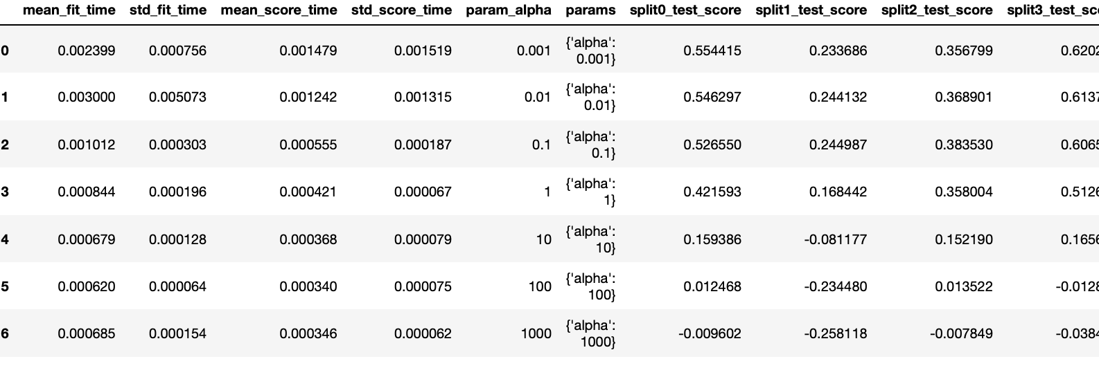
- multiprocessing을 이용한 GridSearchCV
import multiprocessing #모델을 페럴하게 사용하기위해
from sklearn.datasets import load_iris
from sklearn.linear_model import LogisticRegression

iris = load_iris()

param_grid = [{'penalty' : ['l1','l2'],
               'C' : [0.5, 1.0, 1.5, 1.8, 2.0, 2.4]}]

gs = GridSearchCV(estimator=LogisticRegression(), param_grid=param_grid,
					scoring='accuracy', cv=10, n_jobs=multiprocessing.cpu_count())

result = gs.fit(iris.data, iris.target)

print("최적 점수 : {}".format(reshlt.best_score_))
print("최적 파라미터 : {}".format(result.best_params_))
print(gs.best_estimator_)

# 최적 점수 : 0.9800000000000001
# 최적 파라미터 : {'C': 2.4, 'penalty': 'l2'}
# LogisticRegression(C=2.4)

pd.DataFrame(result.cv_results_)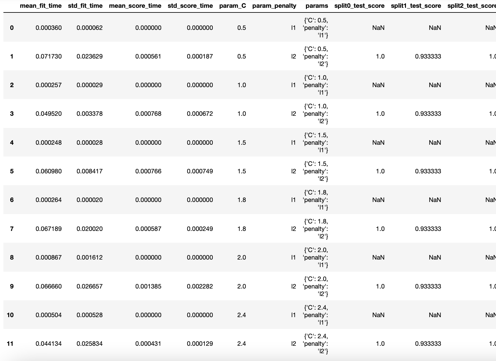
preprocessing 데이터 전처리 모듈
- 데이터의 특징 스케일링(feature scaling)을 위한 방법으로 표준화(Standardization)와 정규화(Normalization) 사용
- 표준화 방법

- 정규화 방법

- scikit-learn에서는 개별 벡터 크기를 맞추는 형태로 정규화
StandardScaler: 표준화 클래스
iris = load_iris()
iris_df = pd.DataFrame(data=iris.data, columns = iris.feature_names)
iris_df.describe()
from sklearn.preprocessing import StandardScaler

scaler = StandardScaler()
iris_scaled = scaler.fit_transform(iris_df)
# fit를 통해 정규화된 정보를 가져오고 / transform을 통해 스케일된 변환을 거친다.
iris_df_scaled = pd.DataFrame(data=iris_scaled, columns=iris.feature_names)

iris_df_scaled.describe()
X_train, X_test, y_train, y_test = train_test_split(iris_df_scaled, iris.target, test_size=0.3)

model = LogisticRegression()
model.fit(X_train, y_train)

print("훈련 데이터 점수 : {}".format(model.score(X_train, y_train)))
print("평가 데이터 점수 : {}".format(model.score(X_test, y_test)))

# 훈련 데이터 점수 : 0.9809523809523809
# 평가 데이터 점수 : 0.9111111111111111
MinMaxScaler: 정규화 클래스
from sklearn.preprocessing import MinMaxScaler

scaler = MinMaxScaler()
iris_scaled = scaler.fit_transform(iris_df)
iris_df_scaled = pd.DataFrame(data=iris_scaled, columns=iris.feature_names)
iris_df_scaled.describe()
X_train, X_test, y_train, y_test = train_test_split(iris_df_scaled, iris.target, test_size=0.3)

model = LogisticRegression()
model.fit(X_train, y_train)

print("훈련 데이터 점수 : {}".format(model.score(X_train, y_train)))
print("평가 데이터 점수 : {}".format(model.score(X_test, y_test)))

# 훈련 데이터 점수 : 0.9142857142857143
# 평가 데이터 점수 : 0.9333333333333333
성능 평가 지표
정확도(Accuracy)
- 정확도는 전체 예측 데이터 건수 중 예측 결과가 동일한 데이터 건수로 계산
- scikit-learn에서는 accuracy_score 함수를 제공
- 정확도만 보고 이 데이터의 신뢰도를 정확히 알 수는 없다.
from sklearn.datasets import make_classification  #데이터를 만드는 모듈
from sklearn.linear_model import LogisticRegression
from sklearn.matrics import accuracy_score

X, y = make_classification(n_samples=1000, n_features=2, n_informative=2,
  				n_redundant=0, n_clusters_per_class=1)
#샘플은 1000개 / feature은 2개  / 의미있는 feature가 2개  /  노이즈가 0  / 클래스당 클러스터가 1개

X_train, X_test, y_train, y_test = train_test_split(X, y, test_size=0.3)

model = LogisticRegression()
model.fit(X_train, y_train)

print("훈련 데이터 점수 : {}".format(model.score(X_train, y_train)))
print("평가 데이터 점수 : {}".format(model.score(X_test, y_test)))

# 훈련 데이터 점수 : 0.9814285714285714
# 평가 데이터 점수 : 0.9766666666666667

predict = model.predict(X_test)
print("정확도 : {}".format(accuracy_score(y_test, predict)))

# 정확도 : 0.9766666666666667
오차 행렬(Confusion Matrix)
- True Negative: 예측값을 Negative 값 0으로 예측했고, 실제 값도 Negative 값 0
- False Positive: 예측값을 Positive 값 1로 예측했는데, 실제 값은 Negative 값 0
- False Negative: 예측값을 Negative 값 0으로 예측했는데, 실제 값은 Positive 값 1
- True Positive: 예측값을 Positive 값 1로 예측했고, 실제 값도 Positive 값 1
from cklearn.metrics import confusion_matrix

confmat = confusion_matrix(y_true=y_test, y_pred=predict)
print(confmat)

# [[142   7]
#  [  0 151]]

fig, ax = plt.subplots(figsize = (2.5, 2.5))
ax.matshow(confmat, cmap=plt.cm.Blues, alpha=0.3)
for i in range(confmat.shape[0]):
    for j in range(confmat.shape[1]):
        ax.text(x=j, y=i, s=confmat[i,j], va='center', ha='center')

plt.xlabel('predicted label')
plt.ylabel('True label')
plt.tight_layout()
plt.show()
정밀도(Precision)와 재현율(Recall)
- 정밀도 = TP / (FP + TP)
- 재현율 = TP / (FN + TP)
- 정확도 = (TN + TP) / (TN + FP + FN + TP)
- 오류율 = (FN + FP) / (TN + FP + FN + TP)
from sklearn.metrics import precision_score, recall_score

precision = precision_score(y_test, predict)
recall = recall_score(y_test, predict)

print("정밀도 : {}".format(precision))
print("재현율 : {}".format(recall))

# 정밀도 : 0.9556962025316456
# 재현율 : 1.0
F1 Score(F-measure)
- 정밀도와 재현율을 결합한 지표
- 정밀도와 재현율이 어느 한쪽으로 치우치지 않을 때 높은 값을 가짐

from sklearn.metrics import f1_score

f1 = f1_score(y_test, predict)

print("F1 Score : {}".format(f1))

# F1 Score : 0.9773462783171522
ROC 곡선과 AUC
- ROC 곡선은 FPR(False Positive Rate)이 변할 때 TPR(True Positive Rate)이 어떻게 변하는지 나타내는 곡선
- TPR(True Positive Rate): TP / (FN + TP), 재현율
- TNR(True Negative Rate): TN / (FP + TN)
- FPR(False Positive Rate): FP / (FP + TN), 1 - TNR
- AUC(Area Under Curve) 값은 ROC 곡선 밑에 면적을 구한 값 (1이 가까울수록 좋은 값)
from sklern.metrics import roc_curve

pred_proba_class1 = model.predict_proba(X_test)[:,1]
fprs, tprs, thresholds = roc_curve(y_test, pred_proba_class1)

plt.plot(fprs, tprs, label='ROC')
plt.plot([0,1], [0,1], '--k', label='Random')
start, end = plt.xlim()
plt.xticks(np.round(np.arange(start, end, 0.1), 2))
plt.xlim(0,1)
plt.ylim(0,1)
plt.xlabel('FPR')
plt.ylabel('TPR')
plt,legend()
from sklearn.metrics import roc_auc_score

roc_auc = roc_auc_score(y_test, predict)

print("ROC AUC Score : {}".format(roc_auc))

# ROC AUC Score : 0.963309480421352'Youtube > 머신러닝' 카테고리의 다른 글
| [머신러닝] #6 최근접 이웃(K Nearest Neighbor) (0) | 2021.12.27 |
|---|---|
| [머신러닝] #5 서포트 벡터 머신 (0) | 2021.12.22 |
| [머신러닝] #4 로지스틱회귀 (0) | 2021.12.21 |
| [머신러닝] #3 선형 모델 Linear Models (0) | 2021.12.20 |
| [머신러닝] #1 Machine Learning 개념 (0) | 2021.12.20 |