[머신러닝] #6 최근접 이웃(K Nearest Neighbor)

뚠뚠이뚠뚠이 2021. 12. 27. 10:13

2021. 12. 27. 10:13

### 2021.12.23

최근접 이웃(K-Nearest Neighbor)

특별한 예측 모델 없이 가장 가까운 데이터 포인트를 기반으로 예측을 수행하는 방법
분류와 회귀 모두 지원

import pandas as pd
import numpy as np
import multiprocessing
import matplotlib.pyplot as plt
plt.style.use(['seaborn-whitegrid'])

from sklearn.neighbors import KNeighborsClassifier, KNeighborsRegressor
from sklearn.manifold import TSNE
from sklearn.datasets import load_iris, load_breast_cancer
from sklearn.datasets import load_boston, fetch_california_housing
from sklearn.model_selection import train_test_split, cross_validate, GridSearchCV
from sklearn.preprocessing import StandardScaler
from sklearn.pipeline import make_pipeline, Pipeline

K 최근접 이웃 분류

입력 데이터 포인트와 가장 가까운 k개의 훈련 데이터 포인트가 출력
k개의 데이터 포인트 중 가장 많은 클래스가 예측 결과

붓꽃 데이터

#In[]
iris = load_iris()

iris_df = pd.DataFrame(data=iris.data, columns=iris.feature_names)
iris_df['Target'] = iris.target
iris_df

#Out[]

#In[]
X, y = load_iris(return_X_y=True)
X_train, X_test, y_train, y_test = train_test_split(X,y,test_size=0.2)

scaler = StandardScaler()
X_train_scale = scaler.fit_transform(X_train)
X_test_scale = scaler.transform(X_test)

model = KNeighborsClassifier()
model.fit(X_train, y_train)

#Out[]
KNeighborsClassifier()

데이터 전처리전 점수

#In[]
print("학습 데이터 점수 : {}".format(model.score(X_train, y_train)))
print("평가 데이터 점수 : {}".format(model.score(X_test, y_test)))

학습 데이터 점수 : 0.9583333333333334
평가 데이터 점수 : 1.0

데이터 전처리후 점수

#In[1]
model = KNeighborsClassifier()
model.fit(X_train_scale, y_train)

#Out[1]
KNeighborsClassifier()

#In[2]
print("학습 데이터 점수 : {}".format(model.score(X_train_scale, y_train)))
print("평가 데이터 점수 : {}".format(model.score(X_test_scale, y_test)))

#Out[2]
학습 데이터 점수 : 0.9583333333333334
평가 데이터 점수 : 0.9666666666666667

#In[]
cross_validate(estimator=KNeighborsClassifier(),
              X=X, y=y,
              cv=5,
              n_jobs=multiprocessing.cpu_count(),
              verbose=True)
              
#Out[]
{'fit_time': array([0.00156212, 0.00154233, 0.00200725, 0.00164413, 0.00190806]),
 'score_time': array([0.004287  , 0.00399184, 0.00413203, 0.00383401, 0.00303102]),
 'test_score': array([0.96666667, 1.        , 0.93333333, 0.96666667, 1.        ])}

#In[]
param_grid = [{'n_neighbors' : [3,5,7],
              'weights' : ['uniform','distance'],
              'algorithm' : ['ball_tree', 'kd_tree', 'brute']}]
              
gs = GridSearchCV(estimator = KNeighborsClassifier(),
                 param_grid = param_grid,
                 n_jobs=multiprocessing.cpu_count(),
                 verbose=True)
                 
gs.fit(X,y)

#Out[]
Fitting 5 folds for each of 18 candidates, totalling 90 fits
GridSearchCV(estimator=KNeighborsClassifier(), n_jobs=4,
             param_grid=[{'algorithm': ['ball_tree', 'kd_tree', 'brute'],
                          'n_neighbors': [3, 5, 7],
                          'weights': ['uniform', 'distance']}],
             verbose=True)

#In[]
print(gs.best_estimator_)
print(gs.best_score_)
print(gs.best_params_)

#Out[]
KNeighborsClassifier(algorithm='ball_tree', n_neighbors=7)
0.9800000000000001
{'algorithm': 'ball_tree', 'n_neighbors': 7, 'weights': 'uniform'}

시각화를 위한 함수 설정

#In[]
def make_meshgrid(x,y,h=.02):
    x_min, x_max = x.min()-1, x.max()+1
    y_min, y_max = y.min()-1, y.max()+1
    xx, yy = np.meshgrid(np.arange(x_min, x_max, h),
                        np.arange(y_min, y_max, h))
    
    return xx, yy
    
def plot_contours(clf, xx, yy, **params):
    Z = clf.predict(np.c_[xx.ravel(), yy.ravel()])
    Z = Z.reshape(xx.shape)
    out = plt.contourf(xx, yy, Z, **params)
    
    return out

#In[]
#저차원 변환
tsne = TSNE(n_components=2)
X_comp = tsne.fit_transform(X)

iris_comp_df = pd.DataFrame(data=X_comp)
iris_comp_df['Target'] = y
iris_comp_df

#Out[]

#In[]
plt.scatter(X_comp[:,0], X_comp[:, 1],
           c=y, cmap=plt.cm.coolwarm, s=20, edgecolors='k')
           
#Out[]

#In[]
model = KNeighborsClassifier()
model.fit(X_comp, y)
predict = model.predict(X_comp)

xx, yy = make_meshgrid(X_comp[:,0], X_comp[:,1])
plot_contours(model, xx, yy, cmap=plt.cm.coolwarm, alpha=0.8)
plt.scatter(X_comp[:,0], X_comp[:,1], c=y, cmap=plt.cm.coolwarm, s=20, edgecolors='k')

#out[]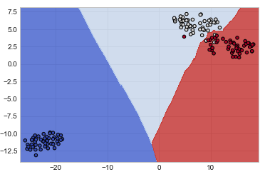

유방암 데이터

#In[]
cancer = load_breast_cancer()

cancer_df = pd.DataFrame(data=cancer.data, columns=cancer.feature_names)
cancer_df['target'] = cancer.target
cancer_df

#Out[]

train data, test data 분리!

#In[]
X, y = cancer.data, cancer.target
X_train, X_test, y_train, y_test = train_test_split(X, y, test_size=0.2)

cancer_train_df = pd.DataFrame(data=X_train, columns=cancer.feature_names)
cancer_train_df['target'] = y_train
cancer_train_df

#Out[]

#In[]
cancer_test_df = pd.DataFrame(data=X_test, columns=cancer.feature_names)
cancer_test_df['target'] = y_test
cancer_test_df

#Out[]

데이터 전처리 전 점수 / 후 점수

#In[1]
scaler = StandardScaler()
X_train_scale = scaler.fit_transform(X_train)
X_test_scale = scaler.transform(X_test)

model = KNeighborsClassifier()
model.fit(X_train, y_train)

#Out[1]

#In[2]
print("학습 데이터 점수 : {}".format(model.score(X_train, y_train)))
print("평가 데이터 점수 : {}".format(model.score(X_test, y_test)))

#Out[2]
학습 데이터 점수 : 0.9516483516483516
평가 데이터 점수 : 0.9035087719298246

#In[1]
model = KNeighborsClassifier()
model.fit(X_train_scale, y_train)

#Out[1]
KNeighborsClassifier()

#In[2]
print("학습 데이터 점수 : {}".format(model.score(X_train_scale, y_train)))
print("평가 데이터 점수 : {}".format(model.score(X_test_scale, y_test)))

#Out[2]
학습 데이터 점수 : 0.978021978021978
평가 데이터 점수 : 0.9473684210526315

모델링

#In[]
estimator = make_pipeline(StandardScaler(),KNeighborsClassifier())

cross_validate(estimator=estimator,
              X=X, y=y,
              cv=5,
              n_jobs=multiprocessing.cpu_count(),
              verbose=True)
              
#Out[]
{'fit_time': array([0.00185204, 0.00381184, 0.00253701, 0.00249338, 0.00242305]),
 'score_time': array([0.00689292, 0.01440096, 0.012604  , 0.01277781, 0.01411605]),
 'test_score': array([0.96491228, 0.95614035, 0.98245614, 0.95614035, 0.96460177])}

#In[]
pipe = Pipeline(
    [('scaler', StandardScaler()),
     ('model', KNeighborsClassifier())])
     
param_grid = [{'model__n_neighbors' : [3,5,7],
              'model__weights' : ['uniform', 'distance'],
              'model__algorithm' : ['ball_tree', 'kd_tree', 'brute']}]
              
gs = GridSearchCV(estimator = pipe,
                 param_grid = param_grid,
                 n_jobs=multiprocessing.cpu_count(),
                 verbose=True)

#In[]
gs.fit(X,y)

#Out[]
Fitting 5 folds for each of 18 candidates, totalling 90 fits
Out[64]:
GridSearchCV(estimator=Pipeline(steps=[('scaler', StandardScaler()),
                                       ('model', KNeighborsClassifier())]),
             n_jobs=4,
             param_grid=[{'model__algorithm': ['ball_tree', 'kd_tree', 'brute'],
                          'model__n_neighbors': [3, 5, 7],
                          'model__weights': ['uniform', 'distance']}],
             verbose=True)

#In[]
print(gs.best_estimator_)
print(gs.best_score_)
print(gs.best_params_)

#Out[]
Pipeline(steps=[('scaler', StandardScaler()),
                ('model',
                 KNeighborsClassifier(algorithm='ball_tree', n_neighbors=7))])
0.9701288619779538
{'model__algorithm': 'ball_tree', 'model__n_neighbors': 7, 'model__weights': 'uniform'}

시각화

#In[]
tsne = TSNE(n_components=2)
X_comp = tsne.fit_transform(X)

cancer_comp_df = pd.DataFrame(data=X_comp)
cancer_comp_df['target'] = y
cancer_comp_df

#Out[]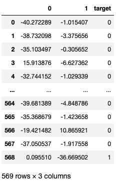

#In[]
plt.scatter(X_comp[:,0], X_comp[:,1], c=y, cmap=plt.cm.coolwarm, s=20, edgecolors='k')

#Out[]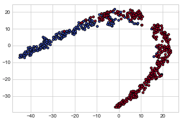

#In[]
model = KNeighborsClassifier()
model.fit(X_comp, y)
predict = model.predict(X_comp)

xx, yy = make_meshgrid(X_comp[:, 0], X_comp[:,1])
plot_contours(model, xx, yy, cmap=plt.cm.coolwarm, alpha=0.8)
plt.scatter(X_comp[:,0], X_comp[:, 1], c=y, cmap=plt.cm.coolwarm, s=20, edgecolors='k')

#Out[]

k 최근접 이웃 회귀

k 최근접 이웃 분류와 마찬가지로 예측에 이웃 데이터 포인트 사용
이웃 데이터 포인트의 평균이 예측 결과

보스턴 주택 가격 데이터

#In[]
boston = load_boston()

boston_df = pd.DataFrame(data=boston.data, columns=boston.feature_names)
boston_df["TARGET"] = boston.target
boston_df

#Out[]

데이터 전처리 전 점수 / 후 점수

#In[1]
scaler = StandardScaler()
X_train_scale = scaler.fit_transform(X_train)
X_test_scale = scaler.transform(X_test)

model = KNeighborsRegressor()
model.fit(X_train, y_train)

#Out[1]
KNeighborsRegressor()

#In[2]
print("학습 데이터 점수 : {}".format(model.score(X_train, y_train)))
print("평가 데이터 점수 : {}".format(model.score(X_test, y_test)))

#Out[2]
학습 데이터 점수 : 0.6850536552455034
평가 데이터 점수 : 0.44632061414558033

#In[1]
model = KNeighborsRegressor()
model.fit(X_train_scale, y_train)

#Out[1]
KNeighborsRegressor()

#In[2]
print("학습 데이터 점수 : {}".format(model.score(X_train_scale, y_train)))
print("평가 데이터 점수 : {}".format(model.score(X_test_scale, y_test)))

#Out[2]
학습 데이터 점수 : 0.8399528467697587
평가 데이터 점수 : 0.7240482286290111

모델링

#In[]
estimator = make_pipeline(StandardScaler(),KNeighborsRegressor())

cross_validate(estimator=estimator,
              X=X, y=y,
              cv=5,
              n_jobs=multiprocessing.cpu_count(),
              verbose=True)
              
#Out[]
{'fit_time': array([0.00622606, 0.00805902, 0.00620103, 0.00619411, 0.00268173]),
 'score_time': array([0.00342488, 0.00330806, 0.00353193, 0.00340295, 0.00339413]),
 'test_score': array([0.56089547, 0.61917359, 0.48661916, 0.46986886, 0.23133037])}

#In[]
pipe = Pipeline(
    [('scaler', StandardScaler()),
     ('model', KNeighborsRegressor())])
     
param_grid = [{'model__n_neighbors' : [3,5,7],
              'model__weights' : ['uniform', 'distance'],
              'model__algorithm' : ['ball_tree', 'kd_tree', 'brute']}]
              
gs = GridSearchCV(estimator = pipe,
                 param_grid = param_grid,
                 n_jobs=multiprocessing.cpu_count(),
                 verbose=True)

#In[]
gs.fit(X,y)

#Out[]
Fitting 5 folds for each of 18 candidates, totalling 90 fits
Out[110]:
GridSearchCV(estimator=Pipeline(steps=[('scaler', StandardScaler()),
                                       ('model', KNeighborsRegressor())]),
             n_jobs=4,
             param_grid=[{'model__algorithm': ['ball_tree', 'kd_tree', 'brute'],
                          'model__n_neighbors': [3, 5, 7],
                          'model__weights': ['uniform', 'distance']}],
             verbose=True)

#In[]
print(gs.best_estimator_)
print(gs.best_score_)
print(gs.best_params_)

#Out[]
Pipeline(steps=[('scaler', StandardScaler()),
                ('model',
                 KNeighborsRegressor(algorithm='ball_tree', n_neighbors=7,
                                     weights='distance'))])
0.4973060611762845
{'model__algorithm': 'ball_tree', 'model__n_neighbors': 7, 'model__weights': 'distance'}

시각화

#In[]
tsne = TSNE(n_components=1)
X_comp = tsne.fit_transform(X)

boston_comp_df = pd.DataFrame(data=X_comp)
boston_comp_df['target'] = y
boston_comp_df

#Out[]

#In[]
plt.scatter(X_comp, y, c='b', cmap=plt.cm.coolwarm, s=20, edgecolors='k')

#Out[]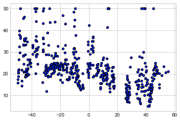

#In[]
model = KNeighborsRegressor()
model.fit(X_comp, y)
predict = model.predict(X_comp)

plt.scatter(X_comp, y, c='b', cmap=plt.cm.coolwarm, s=20, edgecolors='k')
plt.scatter(X_comp, predict, c='r', cmap=plt.cm.coolwarm, s=20, edgecolors='k')

#Out[]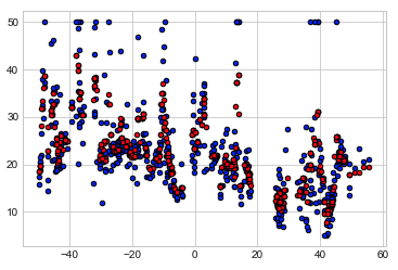

'Youtube > 머신러닝' 카테고리의 다른 글

[머신러닝] #7 나이브 베이즈 분류 (0)	2021.12.27
[머신러닝] #5 서포트 벡터 머신 (0)	2021.12.22
[머신러닝] #4 로지스틱회귀 (0)	2021.12.21
[머신러닝] #3 선형 모델 Linear Models (0)	2021.12.20
[머신러닝] #2 Scikits-learn (0)	2021.12.20

내 블로그 - 관리자 홈 전환	`Q` `Q`
새 글 쓰기	`W` `W`

글 수정 (권한 있는 경우)	`E` `E`
댓글 영역으로 이동	`C` `C`

이 페이지의 URL 복사	`S` `S`
맨 위로 이동	`T` `T`
티스토리 홈 이동	`H` `H`
단축키 안내	`Shift` + `/` `⇧` + `/`

Changhyoni_developer

[머신러닝] #6 최근접 이웃(K Nearest Neighbor)

최근접 이웃(K-Nearest Neighbor)

K 최근접 이웃 분류

붓꽃 데이터

유방암 데이터

k 최근접 이웃 회귀

보스턴 주택 가격 데이터

'Youtube > 머신러닝' 카테고리의 다른 글

+ Recent posts

티스토리툴바

단축키

내 블로그

블로그 게시글

모든 영역